Model of Maximum Load on a Distributed Cache (Non-Uniform Access Patterns)

In a previous post I discussed the maximum gap of draws from $U\Big(0, 1)^{n}$. There is a clear application of this problem to load balancing across many nodes. Given a dataset ($X$) of $d$ keys randomly hashed to one of $n$ nodes, we can expect that no node is responsible for more than $\sim d\log\Big(n)/n$ keys. However, requests are not distributed equally across keys. A node storing a few popular keys may have much higher load than a node storing hundreds of less frequently accessed keys. Today we’ll calculate a bound for max load ($M$) assuming keys an arbitrary distribution over $X$ and that keys are assigned to nodes at random with a hash function, $h\colon X \to [1, n]$.

Because the standard Pareto distribution doesn’t have an $n^{th}$ moment when $\alpha \lt n$ we’ll prefer the more complicated-looking, but much friendlier alternative. The truncated Pareto also maps onto the concept of a dataset with known size (i.e. $d \leftrightarrow H$) quite well.

I’ll use the truncated Pareto distribution as a concrete example, although the bounds given will apply for any distribution. The density of a truncated Pareto defined on $\Big[1, H]$ is as follows.

$$\begin{equation} f_{\alpha, H}\Big(x) = {\frac {\alpha x^{-\alpha-1}}{1-{H}^{-\alpha}}} \ , \ \alpha > 0 \end{equation}$$

We can find a loose upper bound on $M$ by assuming the most frequently accessed keys all hash to a single node. This event occurs with very low probability (i.e. $n^{-\lceil d\log\Big(n)/n \rceil} \approx 0$) and isn’t all that useful.

$$\begin{equation} M \leq \int_{1}^{\lceil d\log\Big(n)/n \rceil} f_{\alpha, d}\Big(x) \ dx \ \qquad \textit{w.v.h.p} \end{equation}$$

I was quite proud of myself for this idea! Too big for my britches again.

Alternatively, we can treat $\textbf{density}$ as a random variable and estimate the mean and variance of the $\textbf{density}$ over $\Big[1, d]$. From there we can bound $M$ by bounding the total load generated by some number of instances of a random variable with the following properties:

$$\begin{equation} \begin{aligned} E\Big[f_{\alpha, d}\Big(x)] & \approx & \frac{1}{d} \int_{1}^{d} f_{\alpha, d}\Big(x) \ dx = \frac{1}{d} \\ \text{Var}\Big[f_{\alpha, d}\Big(x)] & \approx & \int_{1}^{d} \left(f_{\alpha, d}\Big(x) - \frac{1}{d}\right)^2 \ dx \end{aligned} \end{equation}$$

This approach might be viable given a distribution with faster decaying tails, but in this case it produced a variance too high to be of any use. In general, methods that try to find $M$ by bounding the load on a fixed number of keys also consider the event that other nodes with fewer keys exceed that bound as well. This gets dodgy very quickly, I want no parts of it.

The most successful approach I tried involved re-framing the problem to focus more on load attributable to each node rather than sums of keys’ request frequencies. Consider a collection of $n$ functions $g_j \colon \{0, 1\}^d \to \Big[0, 1]$. Each function takes arguments corresponding to whether the $1^{st}, 2^{nd}, \ldots, d^{th}$ key hashes to the $j^{th}$ node and returns the load on that node. For a discrete distribution over $X$ we’ll define $g_j$ as follows:

For continous distributions we can define $f\big(x_i)$ in terms of the difference in the CDF. i.e. $f\big(x_i) \approx F\Big({x_i + 1}) - F\Big({x_i})$;

$$\begin{equation} g_j\big(\{0, 1\}^{d}) = \sum_{i=1}^{d} f\big(x_i) \cdot \mathbb{1}\big[h\big({x_i}) = j] \end{equation}$$

The following two properties then make it possible to apply McDairmid’s inequality on a collection of nodes.

• Our hash function, $h\colon X \to [1, n]$ distributes keys onto nodes $s.t.$ all $\mathbb{1}\big[h\big({x_i}) = j]$ are independent.

• Changing whether or not a single key ($x_i$) hashes onto node $j$ changes the load on $j$ by exactly $\pm f\big(x_i)$.

McDairmid’s inequality (below) allows us to bound each $g_j$ about it’s expectation with tunable certainty, thus we can find an $\epsilon$ sufficiently large that the bound holds with high probability.

$$\begin{equation} P\left[g\big(x_{1},x_{2},\ldots ,x_{d})- E\big[g\big(x_{1},\ldots,x_{d})] \geq \varepsilon \right] \leq e^{-2\varepsilon ^{2} / \sum _{i=1}^{d}f\big(x_{i})^{2}} \end{equation}$$

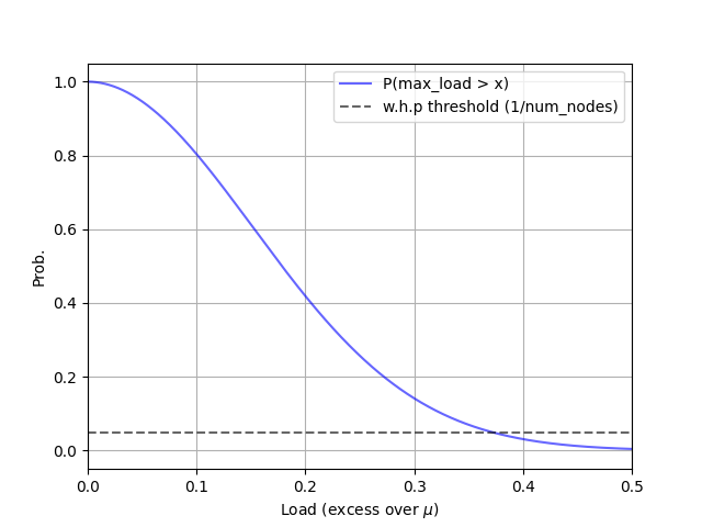
In the diagrams at left I:

1. Calculate an upper bound on $M$ that holds $\textit{w.h.p}$.
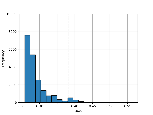
2. Simulate $M$ under Pareto distributed load to verify these results…

# case #1: max. load
d, n, a, mu, p = 2000, 20, 0.4, 1/20, []
t = ss.truncpareto(a, d)
diffs = [
  (t.cdf(x+1)-t.cdf(x))**2 for x in range(1,d+1)
]
for i in range(1,d+1):
   p.append(np.exp(-(2*(i/d)**2)/sum(diffs)))

# case #1 - simulation 
maxes = []
diffs = [
  t.cdf(x+1)-t.cdf(x) for x in range(1,d+1)
]
for j in range(20000):
   ns = collections.defaultdict(np.float64)
   for i, nid in enumerate(
          np.random.randint(0,n,d)
  ):
       ns[nid] += diffs[i]
   maxes.append(sorted(ns.values())[n-1])

$\textbf{N.B.}$ McDairmid’s inequality is closely related to Hoeffeding’s Lemma. While McDairmid’s only requires bounded differences, we have differences that are exclusively $\pm f\Big(x_i)$.

The remainder of this post works through an example using pareto distributed load and $d=2000, \alpha=0.4, n=20$.

$\textbf{Fig. 1}$: Upper Bound of $M$ With Pareto Request Patterns ($M \leq 0.4216 \ \textit{w.h.p}$)

$\textbf{Fig. 2}$: Simulated $M$ With Pareto Request Patterns ($M \approx 0.3889$)

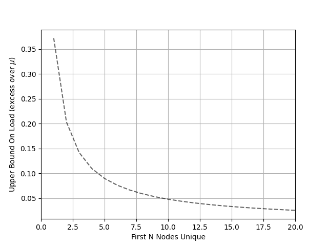
We can construct a tighter bound if we can assume the $c$ most requested keys all hash onto different nodes. Rearranging McDairmid’s inequality gives $M_c^*$, a bound that’s conditioned on this event. To achieve $M_c^*$ the maximum load generated from keys $\Big(c, d\Big]$ must land on the same node as $x_1$. This is quite unlikely.

$$\begin{equation} M_c^* = f\Big(x_1) + \frac{1}{n} + \left( \frac{\log\big(n)}{2} \sum_{i=c}^d f\big(x_i)^2 \right)^{1/2}, \qquad c \in \Big[1, d) \end{equation}$$

$$\begin{equation} Pr\left[M \geq M_c^* \mid \text{top c keys on uniq. nodes} \right] \lt \frac{1}{n^{2}} \end{equation}$$

# case #2: conditional max. load
for i in range(0,n):
  cml = (0.5*np.log(n)*sum(diffs[i:]))**(1/2)
  cmls.append(cml)

$\textbf{Fig. 3}$: Maximum Excess Load Given First $c$ Keys on Unique Nodes $\Big(M_c^*)$