Fixing Redis-Benchmark Again

It’s been a productive last few days thinking about caches (theory, more theory). I haven’t written any code though, let’s change that. Today I’m going to make a $\textit{tiny}$ change to $\texttt{redis-benchmark}$ that will allow me to benchmark with Pareto (or Zipf) distributed traffic. Because web traffic is far more likely to be Pareto (see: FIFO Queues Are All You Need, Table 1) than uniformly distributed, testing a cache under this alternative distribution more closely mimics real request patterns. This was a quick experiment and the change (in it’s entirety!) is below.

$\textbf{N.B}$ — The $\texttt{redis-benchmark}$ defaults (1) maximize entropy, (2) produce larger DBs faster and (3) maximize cache evictions. Recall that $U\Big(0, r)$ is the maximum entropy distribution with support on $\Big[0, r]$. Observations (2) and (3) follow from the fact that each key has $p\big(x_k) \sim 1 - e^{-d/r}$ of occurring in any interval of $d$ operations. If this was intentional, I can see why they’d do this. If not, path of least resistence, whatever…

$\textbf{N.B}$ — Multiple calls to $\texttt{pow}$ are a performance hazard here. Anecdotally, on $\texttt{localhost}$ I was hitting 120,000 - 130,000 rps with either uniform or pareto distributed traffic. It does make a tiny difference, but it won’t overshadow the main point.

@@ -104,6 +104,7 @@ static struct config {
+    double zipf_shape;
 } config;

@@ -378,11 +379,16 @@ static void randomizeClientKey(client c) { 
     for (i = 0; i < c->randlen; i++) {
         char *p = c->randptr[i]+11;
+
         size_t r = 0;
-        if (config.randomkeys_keyspacelen != 0)
-            r = random() % config.randomkeys_keyspacelen;

+        if (config.randomkeys_keyspacelen != 0) {
+            if (config.zipf_shape != 0) {
+                double z = config.zipf_shape;
+                r = (size_t)floor(
+                    pow(1.0 - drand48() * (1 - 1.0 / pow(config.randomkeys_keyspacelen, z)), -1.0 / z)
+                );
+            } else  {
+                r = random() % config.randomkeys_keyspacelen;
+            }
+        }

@@ -1442,6 +1448,8 @@ int parseOptions(int argc, char **argv) {
+        } else if (!strcmp(argv[i],"-z")) {
+            config.zipf_shape = strtod(argv[++i], NULL);

$\textbf{N.B}$ — I refer to $\texttt{cfg.zipf_shape}$ as $\alpha$ and $\texttt{cfg.randomkeys_keyspacelen}$ as $K_{max}$ in the text.

The only meaningful change is in $\texttt{randomizeClientKey}$, where I replace a random key distributed on $U\Big(1, K_{\text{max}})$ with one distributed on $Pa\Big(\alpha)$. I apply the following transformation to $u \sim U\Big(0, 1)$ to produce a Pareto variable with an upper bound at $K_\text{max}$.

$$\begin{equation} k = \left(1 - u\left(1 - \frac{1}{K_{\text{max}}^{\alpha}}\right)\right)^{-1/\alpha} \end{equation}$$

To test that my changes actually worked I ran a few small tests. Results presented below.

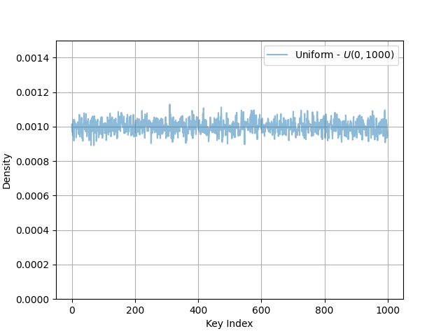
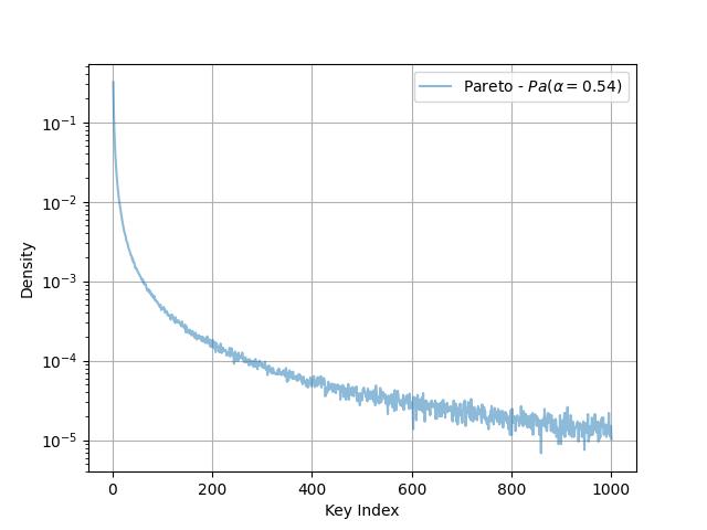
$\textbf{Test 1}$ — I set Redis to AOF mode and fsync’d every 1s. I then wrote a small program to read the AOF and count the frequency of SET operations per key. The leftmost figure shows the results using the original benchmark methodology, the other figure shows the Pareto distributed results generated with the following command:

redis-benchmark -z 0.54 -r 1000 -n 500000 -t SET

Distributions Generated From Uniform & Pareto Benchmarking $(K_{max}=1k ,\ \#Req \sim 500k)$

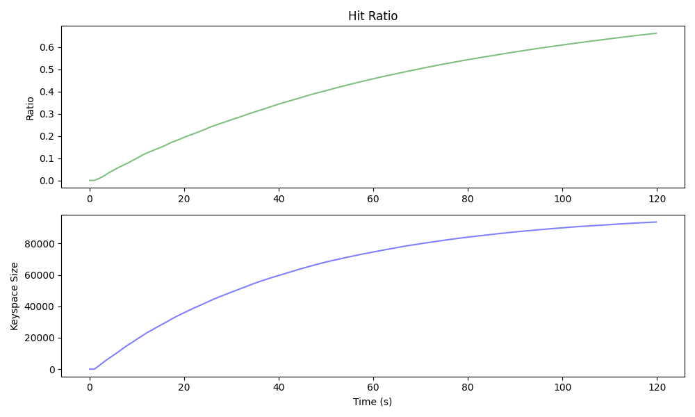
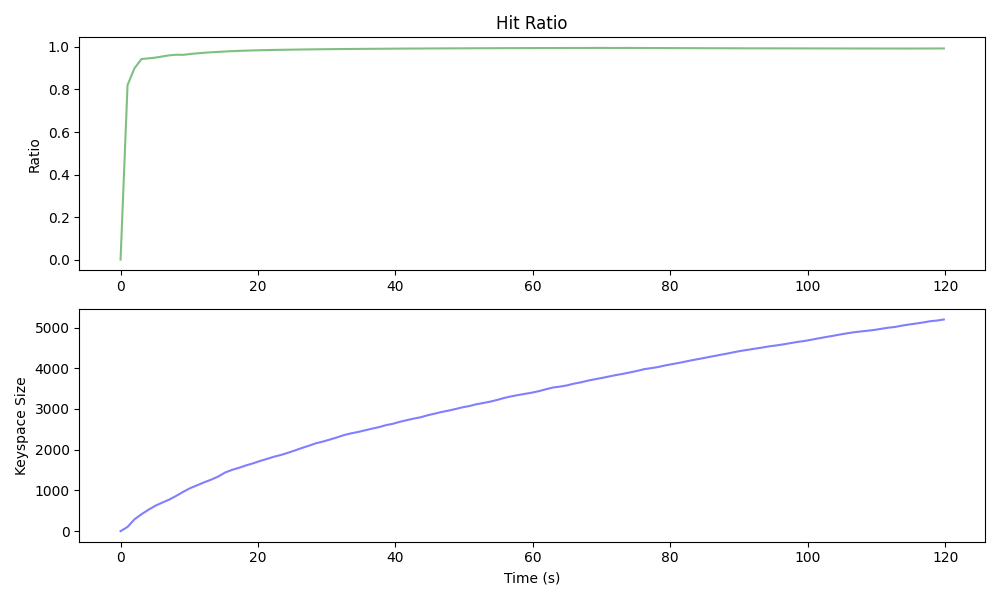
$\textbf{Test 2}$ — I throttled the benchmarking script to $\sim 3000 \text{rps}$ of mixed $\texttt{SET}$ and $\texttt{GET}$ operations and then scraped $\texttt{keyspace_hits}$, $\texttt{keyspace_misses}$, and $\texttt{keys}$ from the target DB. The uniform benchmark produced a DB that grew in size logarithmically and a hit-ratio that mirrored that growth 1:1. The Pareto distributed benchmark (below) produced a much smaller DB and achieved a higher hit-ratio much more quickly.

Uniform Benchmarking $(K_{max}=100k ,\ \#Req \sim 300k)$

Pareto Benchmarking $(K_{max}=100k ,\ \alpha=0.54 ,\ \#Req \sim 300k)$

This addresses just the first of my two gripes with $\texttt{redis-benchmark}$. My second gripe is that it doesn’t allow for correlated requests. In production, one can expect that operations on the same key closely follow one another. Given a stream of keys $k_0, k_1, \dots, k_n$, we should expect $p\Big(k_i = x_j) \leq p\Big(k_i = x_j \mid k_{i-1} = x_j)$.

This is a petty complaint and beefing up a client too much to do more stuff shouldn’t be a bottleneck that limits the efficacy your benchmarking tool. With that said, here’s how I might “fix” $\texttt{redis-benchmark}$…

$\textbf{Fig 1.1}$ — The CDF of Truncated Pareto. Following my first change, we’d map a value from $u \sim U\Big(0, 1)$ to $\Big[1, \infty)$ using the inverse CDF. This figure shows the truncated Pareto with 16 keys and highlights the values of $u$ that correspond to the 3rd key.

$\textbf{Fig. 1}$ — Pareto Distributed Keys

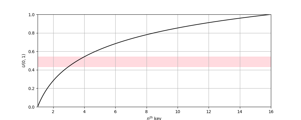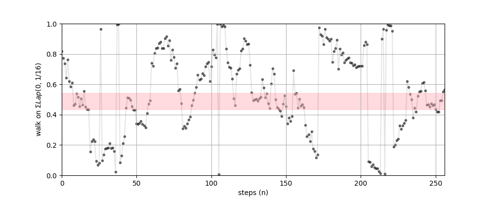
Rather than using $u \sim U\Big(0, 1)$, we’ll generate a random walk on $\Big(0, 1)$. For any key, the probability of being chosen is no longer constant, it’s now a function of the position of the walk $\Big(u_{i - 1})$.

$$\begin{equation} p_k = \int_k^{k+1} f\Big(x) \ dx \ \to \int_{F\Big(k)}^{F\Big({k+1})} g\Big(u_{i - 1}, x) \ dx \end{equation}$$

Where $f\Big(x)$ is the pdf of the Pareto, and $g\Big(u_{i-i}, x)$ is the distribution for the $i^{th}$ step on the walk. In practice, $g$ can be any easy-to-calculate random variable.

$\textbf{Fig 1.2}$ — A random walk on $\Big(0, 1)$ where each step is Laplace distributed w. $g\Big(x) = \operatorname{Lap}\Big(u_{i - 1}, 0.0625)$. Any key is selected with approximately the same frequency as the original method, but selection probability for $k$ is maximized when the walk is near $k$.

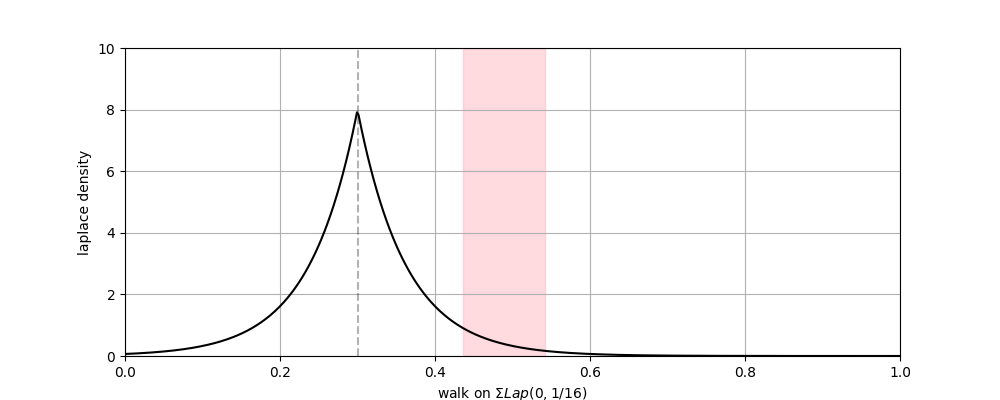
$\textbf{Fig 1.3}$ — The Laplace pdf. The probability the highlighted key is selected is the probability that the walk steps into the relevant range.

$$\begin{equation} \int_{F\Big(k)}^{F\Big({k+1})} \operatorname{Lap}\Big(0.3, 0.0625) \ dx \end{equation}$$

The Laplace is a convenient kernel choice because values are easily generated via. the inverse transform (either directly or difference of two exponential vars).

$\textbf{Fig. 2}$ — Laplace Random Walk over a Keyspace

This is an easy change that should just requires about 10 LOC added to $\texttt{redis-benchmark}$. The next time I need it I’ll try to squeeze this in and see if it gives the desired results.