An Upper Bound For One-Hit Wonder Counts

Although this post is about caching, I’ll ignore specific properties of the cache (e.g. size, eviction method) and focus on getting an upper bound on OHWs.

Today I’m going to find an upper bound on the number of “one-hit wonders” in a stream of requests. Given a set of $n$ keys, we’ll refer to keys that appear exactly once in $m$ requests as “one-hit wonders” (OHW). A high OHW count implies that a cache of these keys is likely filled with items that won’t be requested again. Being able to bound the OHW count is a good prerequisite step before designing a caching algorithm of our own.

We don’t need to limit ourselves to OHWs. A more general notion of efficiency may count the probability that a single key ($x_k$) appears at least once and no more than $h$ times. Assuming a key appears with a corresponding probability $f\Big(x_k)$, the probability it appears more than once, but no more than $h$ times in a stream is as follows:

An even more useful cache efficiency metric could be calculated by estimating a distribution over the number of cache hits, misses or hit-ratio for each key.

$$\begin{equation} \begin{aligned} & E\Big[\#\textit{h-hit wonders}] & = & \sum_{k=1}^n \sum_{j=1}^h Pr\Big(\#x_k = j) \\ & & = & \sum_{k=1}^n \sum_{j=1}^h {{m}\choose{j}} \Big(1 - f\Big(x_k))^{m - j} f\Big(x_k)^{j} \end{aligned} \end{equation}$$

When we restrict this to the OHW case ($j=1$) the expression becomes somewhat easier to work with.

$$\begin{equation} E\Big[\textit{#OHW}] = m \sum_{k=1}^n \Big(1 - f\Big(x_k))^{m - 1} f\Big(x_k) \end{equation}$$

Intuitively, a uniform distribution over all keys seems like a good first guess at maximizing $\#OHW$. In the following section we’ll show that it’s a (near) optimal distribution.

1. Let’s consider an upper bound for a specific distribution over $n$ keys. What is an upper bound on $\#OHW$ if all keys appear with equal probability i.e. $f\Big(x_k) = 1/n$?

$$\begin{equation} E\Big[\textit{#OHW}] = m \sum_{k=1}^n \Big(1 - f\Big(x_k))^{m - 1} f\Big(x_k) = m \Big(1 - 1/n)^{m - 1} \approx me^{-m/n} \end{equation}$$

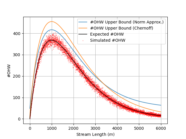
Because each key is equally likely to be an OHW, we can study the tails by approximating $\operatorname{Bin}\Big(n, me^{-m/n}/n)$ to the normal distribution.

Recall that the inverse CDF of $N\Big(\mu, \sigma)$ is $F^{-1}\Big(p) = \mu + \sigma\sqrt{2}\operatorname{erf}^{-1}\Big(2p - 1)$. We replace $\mu = me^{-m/n}, \sigma = \sqrt{n/4}$ to get an upper bound.

$$\begin{equation} \operatorname{Bin}\Big(n, me^{-m/n}/n) \sim N\Big(me^{-m/n}, \sqrt{n \Big(1 - me^{-m/n}/n)\Big(me^{-m/n}/n)}) \end{equation}$$

Assuming an unbounded stream, we won’t know the value of $m$ or $me^{-m/n}/n$, but we can maximize the variance of the distribution by assuming $me^{-m/n}/n = 0.5$. This implies $\sigma^{2}=n/4$ and thus $\#OHW \sim N\Big(me^{-m/n}, \sqrt{n/4})$. We can then reference the inverse CDF of the normal distribution to find a bound that holds with high probability ($p \approx 1 - \frac{1}{n}$).

$$\begin{equation} \textit{#OHW} < me^{-m/n} + \sqrt{2n}/2 \operatorname{erf}^{-1}\Big(1 - 2/n) \qquad \textit{w.h.p} \end{equation}$$

This is a well-known bound for the sum of Bernoulli RVs. A good reference for this inequality is Mitzenmacher (Ch. 4.2). This proof shows this inequality for the more general case of Poisson trials.

Personally, I don’t want to mess around with $\operatorname{erf}^{-1}$. Let’s take a step back and derive a similar upper bound that only uses “nicer” functions. Rather than approximating the sum with the normal distribution, I’ll use a Chernoff Bound for the sum of Bernoulli variables.

$$\begin{equation} {\displaystyle \Pr\Big(X \geq \Big(1 + \delta) \mu )\leq e^{-\delta ^{2}\mu /3},\qquad 0<\delta <1.} \end{equation}$$

To get an upper bound in terms of keys we solve for $\delta$ at some configurable level of certainty (e.g. $1 - 1/n$). This gives:

$$\begin{equation} e^{-\delta ^{2}\mu /3} = 1/n \implies \delta = \sqrt{3\log\Big(n)/\mu} \end{equation}$$

$$\begin{equation} \textit{#OHW} < \left(1 + \sqrt{\frac{3\log\Big(n)}{me^{-m/n}}}\right) me^{-m/n} \qquad \textit{w.h.p} \end{equation}$$

$\textbf{Fig 1.1:}$ — Expected One-Hit Wonders and Bounds (1000 Unique Keys)

$\textbf{Try It Out!}$

s, ohw = 10000, 0
for i in range(10**5):
    a = np.random.choice(
        [0, 1], s, True, [1-1/s, 1/s]
    )
    ohw += (np.count_nonzero(a) == 1)
ohw / int(10**5 * math.exp(-1)) # 0.99932 

2. Can we show that a uniform distribution over $n$ keys actually maximizes $\#OHW$? Does the upper bound from the previous section hold regardless of distribution?

Consider a set of keys with $n = 2$ and a stream of requests with $m = 10000$. If we assign $p_1 = p_2 = 1/2$ we’ll have $\#OHW = 0$ $\textit{w.h.p}$. However, if we set $p_1 = 1/m, p_2 = 1 - 1/m$ we can achieve $E\Big[\#OHW] \approx e^{-1} \approx 0.3678$.

This suggests that on large streams ($m \gg n$) the maximum $\#OHW$ is achieved when $p_1, p_2, \ \dots \ ,p_{n-1} = 1/m, \ p_n=1-n/m$. Intuitively, we can think of this as maximizing each of the first $n - 1$ keys’ probability of one-hitting and then “sacrificing” the $n^{th}$ key.

I could show this more rigorously by setting up the full optimization problem with Lagrange multipliers, but the example at left makes the point clearly enough.

$$\begin{equation} \frac{\delta}{\delta p_j} \left(mp_j\Big(1 - p_j)^{m - 1} \right) = m \Big(1 - p_j)^{m - 2} \Big(mp_j - 1) = 0 \ \implies p_j = 1/m \end{equation}$$

Over a set of $n$ keys this gives a maximum for $E\Big[\#OHW] = n/e$. Slightly modifying our bound from the previous section gives us the following:

$$\begin{equation} \textit{#OHW} < \left(1\ + \sqrt{3e\log\big(n)/n}\right) n/e\ +\ 1 \qquad \textit{w.h.p} \end{equation}$$

Although the key with probability $1 - n/m$ is unlikely to be an OHW I include the $+1$ to be $\textit{extra}$ safe. Regadless, now even if we don’t know $m$ we can bound $\#OHW$ over an arbitrarily long stream provided we know $n$.

3. Now that I’ve done all this work it’s time for the scary part, we must check real data. What are the OHW rates observed in real $\textit{Big Serious Systems}^{TM}$?

Related Reading:

• FIFO Queues are All You Need for Cache Eviction
• SIEVE is Simpler than LRU: an Efficient Turn-Key Eviction Algorithm for Web Caches

In FIFO Queues are All You Need for Cache Eviction, the authors proposed a new class of caching algorithms based on data collected from the traces of several large caching systems.

• From FIFO Queues:

  

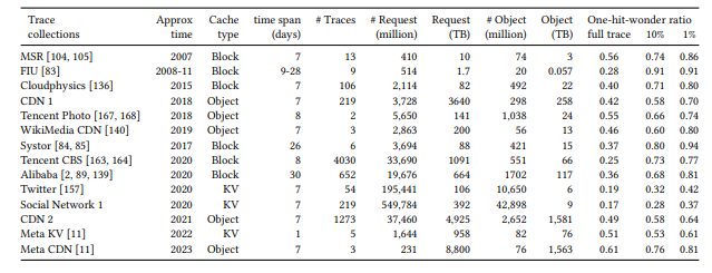
  Our insight is that a cache experiences more one-hit wonders than what common full trace analyses suggested, highlighting the importance of swiftly removing most new objects. Specifically, we observe a median one-hit-wonder ratio of 26% across 6594 production traces”

Rough Sketch — Assume a cache size of $c \lt n$ and an almost uniform distribution (e.g. $p_1...p_{n - 1} = 1/m$). Then at least $\sim n\left(1\ -\ e^{-1}\ - n\sum_{j=1}^{m}\left(\frac{c}{n}\right)^{j}f\big(j)\right)$ keys are never OHWs. Approx $1/e$ are never seen and thus cannot be OHWs (ever elusive!). The distribution of the $\#\textit{req}$ of each of the remaining keys is $f \sim \operatorname{Bin}\Big(m, 1/m)$. We (crudely) assume an LRU eviction algorithm and no temporal correlation s.t. $\big(c/n)$ is the probability of reappearing in the stream of requests before $c$ other unique keys are seen…

This is about what we’d expect based on (2), though perhaps a bit high. If I’ve read the paper correctly there are a few possible reasons for this:

• Their definition of $OHW$ includes items that are requested once and not requested again before being evicted from the cache. I’ve ignored cache capacity $\Big(c)$, but it’s clearly a determining factor. Implicitly, we’ve assumed that $c \gt n, m \gt n$. In practice we’d expect $m > n \gg c$.

• This is a glaring one. The denominator in their OHW ratio $\textit{excludes}$ keys that don’t make an appearance at all. I’ve treated $n$ as a known value, but in practice it’s unlikely the set of keys will be so well defined. This is probably the correct choice and if I followed this convention my estimate would increase to about $e^{-1}/\big(1 - e^{-1}) \approx 0.582$. Yeesh!

Given these caveats and my assumptions, I’m reasonably confident in my upper bound from $\Big(2)$. In practice it seems we can’t avoid specific properties of the cache. A good next step would be to determine the distribution of requests needed to see $k$ unique values given some arbitrary distribution over a set of keys.