Systems…

I worked on a little program yesterday that I’m very excited about. It is a small ($\lt 180$ LOC) Golang package that computes statistical distributions using generating functions. My direct use-case is for modeling components of distributed systems, but in the last 24 hours I’ve found it can be applied to a variety of applications.

$\textbf{N.B}$ — I’m serious about it being small. The code is a GIST available here and also available on my own domain here.

A few weeks ago I realized that histograms produced by metrics and monitoring systems can be treated as probability generating functions (PGFs). Because the distribution of the sum of independent random variables is determined by the product of their PGFs, the product can represent the distribution of the total execution time of sequential calls.

$\textbf{N.B}$ — My previous post was too focused on using mechanical sympathy and statistical approximation to squeeze performance out of an $\mathcal{O}\Big(n^2)$ algorithm. This just isn’t a natural way to model systems. If we’re going through the exercise of modeling systems, we probably don’t care if modeling program returns an answer in milliseconds (not nanoseconds), we likely just want an expressive API and accurate answer.

I previously I described a method for finding a product in $\mathcal{O}\Big(n^2)$ time. That’s OK for small input, but to use higher-fidelity samples, we’ll need a better algorithm for adding PGFs. One foundational result from signal processing is that the Fast-Fourier Transform (FFT) can be used to do polynomial multiplication in $\mathcal{O}\Big(n\ln\Big(n))$ rather than $\mathcal{O}\Big(n^2)$ time. No surprise, if apply FFT to our problem we achieve a similar performance improvement. This is a big step from a sheer computational efficiency perspective, but if we want to model $\underline{\textit{real systems}}$ we need to devise efficient methods to describe a wider set of operations.

To start, we’ll assume a set of $\textit{fundamental operations}$. These are the smallest units of work we’re interested in and we have access to their empirical distributions directly from a metrics collecting system. The code I wrote yesterday gets us closer to modeling $\underline{\textit{real systems}}$ by supporting fast, deterministic calculations for the following functions on fundamental operations.

• $\textbf{Sequential Executions:}$ $\texttt{Seq}\Big(Op, n)$ and $\texttt{SeqMixed}\Big([]Op{...})$ — We calculate the distribution of the end-to-end execution time of $n$ operations. Internally, I use FFT to do this efficiently on large histograms. In practice, we see sub-millisecond responses on histograms with $2^15$ bins.

  $\textbf{Example}$ — Some RPC endpoint makes sequential calls to services $A$, $B$, and $C$. We can calculate the distribution of the total execution time as $\texttt{SeqMixed}\Big(\{Op_a, Op_b, Op_c\})$.

• $\textbf{Parallel Executions:}$ $\texttt{Parallel}\Big(Op, n, k)$ and $\texttt{ParallelMixed}\Big([]Op{...}, k)$ — We calculate the distribution of execution time of the $k^{th}$ of $n$ calls. When making parallel calls of a single operation, we use a result about the distribution of order statistics of the uniform distribution to compute a result in $\mathcal{O}\Big(n)$ time . When making calls to different distributions we use a clever algorithm to compute the result in $\mathcal{O}\Big(nm^2)$ time with $m := length\Big([]Op)$. That may appear ominous, but in practice $m^2$ is often quite small. Testing shows sub-millisecond responses on bins up to $2^15$ and $m \leq 20$.

  $\textbf{Example}$ — We’d like to model a leader election process. We have 9 nodes with different response time characteristics. We have access to each node’s response time distribution as a fundamental operation. We say a leader election is completed after $n/2 + 1$ nodes respond to a message. We could assume all nodes are equivalent and call $\texttt{Parallel}\Big(AvgOp, 5)$. Alternatively, we could call call $\texttt{ParallelMixed}\Big(\{Op_0, Op_1, \ldots Op_8\}, 5)$ to get a more precise result.

Critically, the return types of the functions described above are all just $\texttt{Op}$. This lets us chain arbitrary sets of operations on top of one another to describe more complex system behaviors.

$\textbf{N.B}$ — I need to comment on determinism. Given a system’s fundamental operations, one way to model the execution of higher-level operations could be to simulate paths by drawing a percentile, $u \sim U\Big(0, 1)$ on each fundamental operation in the call-path and transforming that percentile back to milliseconds. Of course, we need to simulate a path many times to get a stable result, but does that really matter? If we really need determinism for this type of exercise is still an open question. I don’t actually think so, but I won’t let that stop me from writing this package…

The following examples show that small programs written with this package can be used to succinctly model hard-to-calculate behaviors in distributed systems. Following each example I simulate the same behavior (via millions of $\texttt{rand()}$ calls) and compare results.

• $\textbf{Leader Election or Synchronous Commit}$ — Let’s study a leader election process similar to the scenario I’ve described above. This pattern could also be used to model the time until a synchronous commit can be acknowledged in a replicated database system.

func main() {

    var distUpperBound = 1 << 10
    var a, b           = 0.0, 0.0
    var alpha, beta    = 15.0, 0.1
    
    // assume response to leader-elections are distributed by the Gamma(alpha, beta). 
    // In practice, we'd pull empirical values from a metrics system, for demonstration
    // any hard-to-work-with distribution will suffice
    d := make(sysmodel.Distribution, distUpperBound)
    gamma := distuv.Gamma{Alpha: alpha, Beta: beta}
    for i := 1; i < distUpperBound; i++ {
        a, b = float64(i), float64(i-1)
        d[i] = gamma.CDF(a) - gamma.CDF(b)
    }

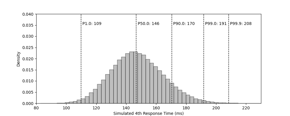
    // Our package calls `Parallel` and requests the distribution of the 4th of 7 nodes to 
    // respond to the election message. It computes the resulting distribution in ~250-300µs.
    result := d.Parallel(7, 4) 
    for _, q := range []float64{0.01, 0.5, 0.90, 0.99, 0.999} {
        soln := result.Percentile(q)
        fmt.Printf("%.3f \t %5d\n", q, soln)
    }
}

• $\textbf{Global Limit Check}$ — Imagine you have a service with regional deployments. Before allowing a user to deploy a resource in one region, you check their total resource usage in all other regions to ensure they’re below a global limit. The regional data-centers are spread all across the world and have radically different response time distributions. The program below models this situation.

$\textbf{N.B}$ - To be honest, I am not totally sure about the implementation of $\texttt{ParallelMixed}$. It seems correct when I test it against some simulations, but there are some scenarios where I’m not “close” to simulation (i.e. $P1$ below). Somewhat concerning, but this is something to improve on. Fingers crossed that I just wrote incorrect simulation code 💀.

func main() {   
    var totNumResponses, reqNumResponses = 7, 7
    var distUpperBound  = 1 << 14
    var a, b            = 0.0, 0.0
    var alpha, beta     = 6.0, 0.3
    
    dists := make([]sysmodel.Distribution, totNumResponses)
    for i := 0; i < totNumResponses; i++ {
        d := make(sysmodel.Distribution, distUpperBound)

        // totally arbitrary responses from each datacenter
        gamma := distuv.Gamma{Alpha: float64(i+2) * alpha, Beta:  beta / float64(i+1)}
        for i := 1; i < distUpperBound; i++ {
            a, b = float64(i), float64(i-1)
            d[i] = gamma.CDF(a) - gamma.CDF(b)
        }
        dists[i] = d
    }

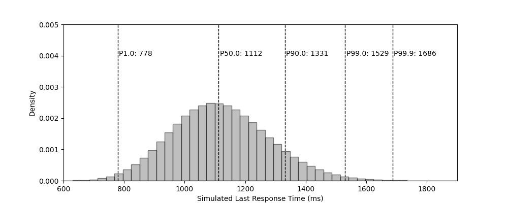
    // calls `sysmodel.ParallelMixed` and requests the distribution of the 7th of 7 nodes,
    // each with a distinct response distributions...
    for _, q := range []float64{0.01, 0.5, 0.90, 0.99, 0.999} {
        result := sysmodel.ParallelMixed(dists, reqNumResponses)
        soln := result.Percentile(q)
        fmt.Printf("%.3f \t %5d\n", q, soln)
    }
}

• $\textbf{Misc. Theoretical Applications}$ — This tool can be used to model more than just calls in distributed systems. Earlier this year I wrote about bounding the growth of a skiplist. In that post, I aimed to find a bound for the distribution of the sum of $n$ geometric distributions with exponentially decreasing rate parameters. Using the traditional methods from probability and TCS, I came up with a bound that I knew was quite loose (off by a factor of $\sim 2x$ for $P99$). However, computing the result via the distributions’ generating functions gives precise results. It’s certainly a $\textit{little}$ motivated by ego, but showing a result through the product of generating functions carries more weight than verifying through simulation.

func skipListSoln(k int, q float64) int {
    var dists          = make([]sysmodel.Distribution, k)
    var a, b           = 0.0, 0.0
    var p              = 0.5
    var distUpperBound = 1 << 15

    for i := 1; i <= k; i++ {
        d := make(sysmodel.Distribution, distUpperBound)
        exp := distuv.Exponential{Rate: math.Pow(p, float64(i))}
        for i := 1; i < distUpperBound; i++ {
            a, b = float64(i), float64(i-1)
            d[i] = exp.CDF(a) - exp.CDF(b)
        }
        dists[i-1] = d
    }

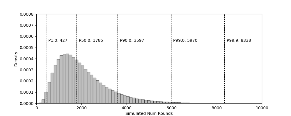
    // calls `sysmodel.Add` and requests the distribution of the sum of the current 
    // distribution and the i^th. Computes these internal additions in <1ms each...
    d := dists[0]
    for i := 1; i < len(dists); i++ {
        d = d.Add(dists[i])
    }
    return d.Percentile(q)
}

func main() {
    var numLevelsTotal = 10
    for _, q := range []float64{0.01, 0.5, 0.90, 0.99, 0.999} {
        soln := skipListSoln(numLevelsTotal, q)
        fmt.Printf("%.2f \t %5d\n", q, soln)
    }
}

$\textbf{Some Limitations...}$

I am quite proud of this work, It’s a lot of thinking to do in one weekend. That said, there are still gaps. I have $\textbf{NOT}$ yet supported (or simply won’t support) the following patterns:

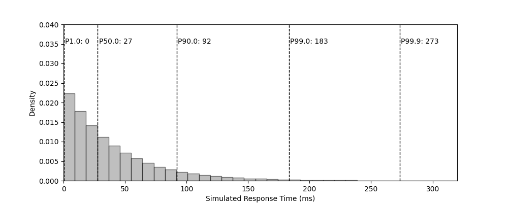
• $\textbf{Randomized Executions:}$ $\texttt{Randomized}\Big(A, Op_B)$ — The number of executions of $\texttt{Op_B}$ is distributed by some other distribution $\texttt{A}$. This can be useful for modeling $\textbf{(1)}$ retry and failure behavior and $\textbf{(2)}$ contingent results. For $\textbf{(1)}$, assume $Op_B$ must be retried $k$ times, where $k \sim A$. For $\textbf{(2)}$, we may wish to model a behavior where $Op_B$ is intentionally called $k \sim A$ times, for example, to return all paginated results. I didn’t include these on my first pass because $A$ isn’t an operation with an execution time, rather it’s just a fact about the system. We can model this behavior, but it will take some additional research. This type of behavior can be thought of as the composition of generating functions $\text{i.e.} \ \varphi_A \circ \varphi_{Op_B}$, see Klenke’s Probability Theory, Thm. 3.8.

  • $\textbf{Update}$ (09/09/24) — Added this! I opted for the naive solution that runs in $\mathcal{O}\left(m n\ln\Big(n)\right)$ where $m := |A|$. There is a better algorithm, but since $m$ is low by design, the naive approach is likely viable. The example below assumes $Op_B \sim \text{Exp}\Big(0.05)$, and retries are distributed geometrically with $p=1/2$. Because these are nice distributions, we can verify the results of $\texttt{Randomized}\Big(A, Op_B)$ analytically by integrating the $\textit{pdf}$ of the Erlang distribution.

  func main() {
      var (
          distUpperBound    = 1 << 12
          maxRetries        = 12.0
          retryDistribution = make(sysmodel.Distribution, int(maxRetries))
          successRate       = 0.5
      )
  
      d := make(sysmodel.Distribution, distUpperBound)
      stdExpon := distuv.Exponential{Rate: 0.05}
      for i := 1; i < distUpperBound; i++ {
          d[i-1] = stdExpon.CDF(float64(i)) - stdExpon.CDF(float64(i-1))
      }
  
      for i := 0; i < len(retryDistribution); i++ {
          retryDistribution[i] = successRate * math.Pow(1-successRate, float64(i))
      }
  
      result := sysmodel.Randomized(retryDistribution, d)
      for _, q := range []float64{0.01, 0.5, 0.90, 0.99, 0.999} {
          soln := result.Percentile(q)
          fmt.Printf("%.3f \t %5d\n", q, soln)
      }
  }

  Percentile	1.0	50.0	90.0	99.0	99.9
  Time (Computed)	0	27	91	182	278
  Time (Simulated)	0	27	92	183	273
  Time (Analytic)	0	27	92	184	283

  

• $\textbf{Correlation}$ — A fundamental assumption of this package is that all responses are independently distributed. It would not be suitable to model the performance of 10,000 concurrent executions against an endpoint that’s not written to support high concurrency. We cannot magically know the resource constrains of a system, I trust the user to apply a $\textit{teensy}$ amount of common sense here…

• $\textbf{Non-Uniform Samples}$ — The FFT depends on uniform sampling. This makes variable-sized buckets from a metrics collection system like Prometheus an invalid choice for seeding a fundamental operation. One could manipulate Prometheus to store $2^15$ values for each histogram, but I suspect many people at your job would be upset with you if you tried.

• $\textbf{Unbounded Variables}$ — This code was written with bounded, discrete distributions in mind. Because I depend on highly-detailed data to form the distributions of fundamental operations, it’s left to the user to graft meaning onto the input data. A natural choice may be “the $j^{th}$ index of the input distribution represents a $j$ millisecond response”, but the code doesn’t enforce this in any way. Additionally, my code makes aggressive optimizations on input distributions with exponentially decreasing tails. If a fundamental distribution is bimodal (e.g. perhaps a call has a timeout at $2^12 \text{ms}$) it’s unlikely to benefit from these shortcuts.