Siphon: Scenario-Analysis In Distributed Systems

$\textbf{TODO}$ — My Taxes. I have to do my taxes before writing up the full results. Sit tight, might be a while, Polymarket has “Dustin Finishes this post by April 30” trading at 12%…

The past month I’ve been developing a method for computing hypothetical latency distributions of calls in distributed systems (e.g. “How would $\texttt{UpstreamSvc.Method}$ respond if the latency distribution of $\texttt{DownstreamSvc.Method}$ were shaped differently?”). In this post, I introduce Siphon, a system that answers these types of performance questions by intercepting Open-Telemetry (OTel) traces and building a call-graph and correlation structure of the system’s components. Specifically, I aimed to achieve four goals:

1. Easy Deployment — Siphon models latency without requiring additional instrumentation. Because Siphon’s ingestion path is implemented as an OTel collector, only configuration changes are required to integrate with Siphon. Many systems, e.g. ORION and WebPerf, both of which require extra instrumentation to make latency predictions.

2. Accurate Forecasts — Siphon implements multiple methods for predicting latency. We observe that for systems under low-to-moderate load, Siphon’s predictions are often within $5\%$ of the target method’s true $p99$ latency.

$\textbf{WARN}$ — Unfortunately, I found that accuracy levels are only possible in extremely specific environments, a failure we will discuss in depth later…

3. Near Real-Time Forecasts — Because Siphon is implemented as part of an OTel pipeline, the latency model can incorporate new data within tens of milliseconds of a span arriving at the collector. In testing, I have found that Siphon can comfortably process $\geq 10,000 \ \text{traces/sec}$ and return queries with a $p99$ around $1s$. Compare this with LatenSeer which only performs analysis offline on a static dataset and processes just $\sim 20$ Twitter $\text{traces/sec}$.

4. Flexible Scenarios — In Siphon, we call a “scenario” a collection of single-node interventions, where each intervention is an affine transform $(aX + b)$ of the latency at node $X$ with constants $a, b \in \big[0, \infty)$.

Although Siphon doesn’t obviate the need for chaos engineering, application profiling, or canary deployments, I believe that (with some work) it may become a handy tool for ad-hoc experimentation and quickly reasoning about the performance of systems. For reasons that will soon become clear, this first attempt at Siphon wasn’t a complete success. This post, therefore, is as much about documenting the research process as introducing a new algorithmic idea.

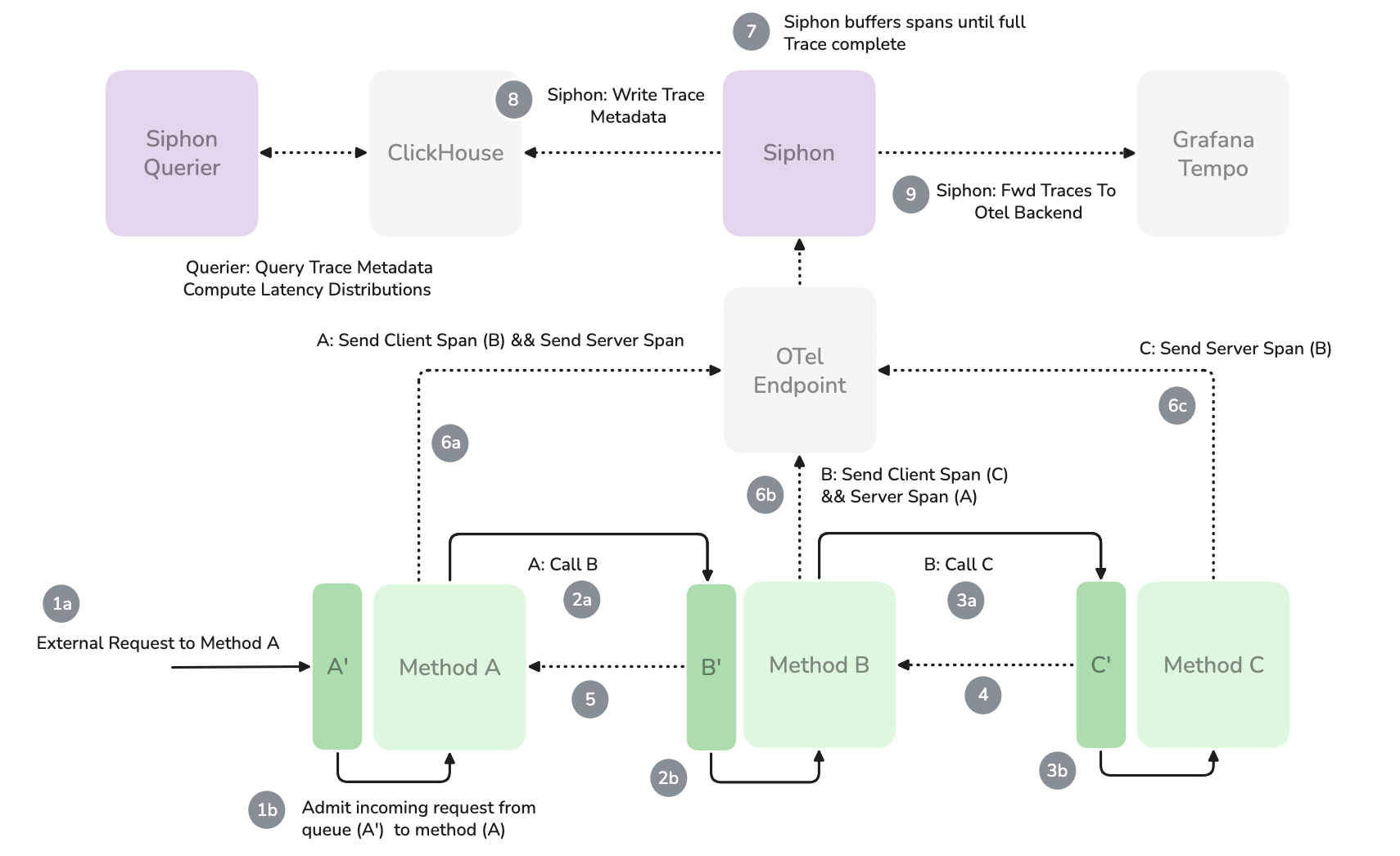
Siphon consists of three components: an OTel collector, a columnar data store, and a querier service. See $\texttt{Fig. 1}$ below.

Fig. 1 — Reference Architecture — (6a), (6b), (6c) All services in a cluster are configured to send all sampled $\texttt{SERVER}$ and $\texttt{CLIENT}$ spans to Siphon. (6a), (7) Siphon buffers spans in memory and only processes complete traces after the root span has been received. (8) Once all of a trace’s spans are available (or a configurable grace period has expired), Siphon computes each service’s execution pattern and exclusive time, and writes a series of records to the data store. (9) Asynchronously, Siphon forwards incoming spans to a traditional OTel exporter (e.g. Tempo, Jaeger).

In the 2000s, systems like Magpie and Sherlock used causal graphs for fault detection and root-cause analysis well before the idea of “distributed tracing” had been popularized. Magpie’s authors posited that “pervasive, online, end-to-end modelling” could be used for capacity planning, probabilistic failure detectors (so-called “Bayesian Watchdogs”), SLA monitoring, and self-tuning systems. In a way, Siphon attempts to realize these possibilities by taking a slightly different approach than similar systems. It differs in two meaningful ways:

• Accounting of Time — Siphon introduces a new metric, $\texttt{exclusive_time}$. Neither $\texttt{response_time}$ nor $\texttt{service_time}$ is sufficiently detailed to act as input in Siphon’s latency model.

$\textbf{N.B}$ — In recent microservices literature it’s become popular to perform offline analysis of traces to build a causal graph (e.g. Palette and TrainTicket). From there, one can “mimic” an application by deploying microservices with similar fanout, execution durations, etc.

• Distributional Estimation — Siphon supports three estimation modes. In two of the three, Siphon fits a lognormal distribution to the per-service distribution of $\texttt{exclusive_time}$. We will soon see that despite its merits, the lognormal distribution cannot capture the long-tailed distribution of exclusive times inherent to distributed systems under load.

I will avoid reviewing the basics of distributed tracing (see: OTel Docs for a refresher). Instead, I will focus on the dummy trace shown in $\texttt{Fig. 2a}$ (JSON) and $\texttt{Fig. 2b}$ (in Grafana UI) to illustrate some of the key concepts in Siphon.

{ // Root Server span, emitted by service A...
  "name": "hello",
  "kind": "SPAN_KIND_SERVER",
  "context": {
    "trace_id": "5b8aa5a2d2c872e8321cf37308d69df2",
    "span_id": "051581bf3cb55c13"
  },
  "parent_id": null,
  "start_time": "2022-04-29T18:52:58.1142Z",
  "end_time": "2022-04-29T18:52:58.1147Z"
}

{ // Client span, emitted by service A, outbound call to B...
  "name": "hello",
  "kind": "SPAN_KIND_CLIENT",
  "context": {
    "trace_id": "5b8aa5a2d2c872e8321cf37308d69df2",
    "span_id": "a1b2c3d4e5f67890"
  },
  "parent_id": "051581bf3cb55c13",
  "start_time": "2022-04-29T18:52:58.1143Z",
  "end_time": "2022-04-29T18:52:58.1146Z"
}

{ // Server span, emitted by service B, inbound from A...
  "name": "hello",
  "kind": "SPAN_KIND_SERVER",
  "context": {
    "trace_id": "5b8aa5a2d2c872e8321cf37308d69df2",
    "span_id": "b3c4d5e6f7a89012"
  },
  "parent_id": "a1b2c3d4e5f67890",
  "start_time": "2022-04-29T18:52:58.1143Z",
  "end_time": "2022-04-29T18:52:58.1145Z"
}

Fig. 2a — Sample Spans — In traditional distributed tracing systems, a $\texttt{SERVER}$ span is associated with the service time of a request and a $\texttt{CLIENT}$ span is associated with the response time of that request from the perspective of the caller.

The first factor that differentiates Siphon from other tools is Siphon’s accounting of time. Siphon introduces a new concept, the exclusive time of a span. Exclusive time approximates the amount of time a service is doing synchronous work. In simple systems, this definition is equivalent to the time a span contributes to the critical path, but that definition does not hold in general. In effect, the exclusive time is the duration where a service has no inflight requests to downstream services. Using the trace in $\texttt{Fig. 2a}$, A’s exclusive time is the sum of two disjoint intervals. First, from 18:52:58.1142 to 18:52:58.1143 (before the call to B) and then from 18:52:58.1146 to 18:52:58.1147 (after the call to B, presumably as it prepares a response to its own caller). To formalize, for $I_A := [A^{\text{start}}, A^{\text{end}})$ and $I_C := [C^{\text{start}}, C^{\text{end}})$:

$$\begin{equation} T_{\text{exc}}(A) := \left| I_A \setminus \bigcup_{C \in \text{children}(A)} I_C \right| \end{equation}$$

These exclusive-time intervals partition the root span’s interval: no two overlap, and together they cover the root exactly. Writing $\text{sub}(A)$ for the set of spans in the subtree rooted at $A$ (including $A$ itself), this gives the accounting identity:

$$\begin{equation} |I_A| = \sum_{X \in \text{sub}(A)} T_{\text{exc}}(X) \end{equation}$$

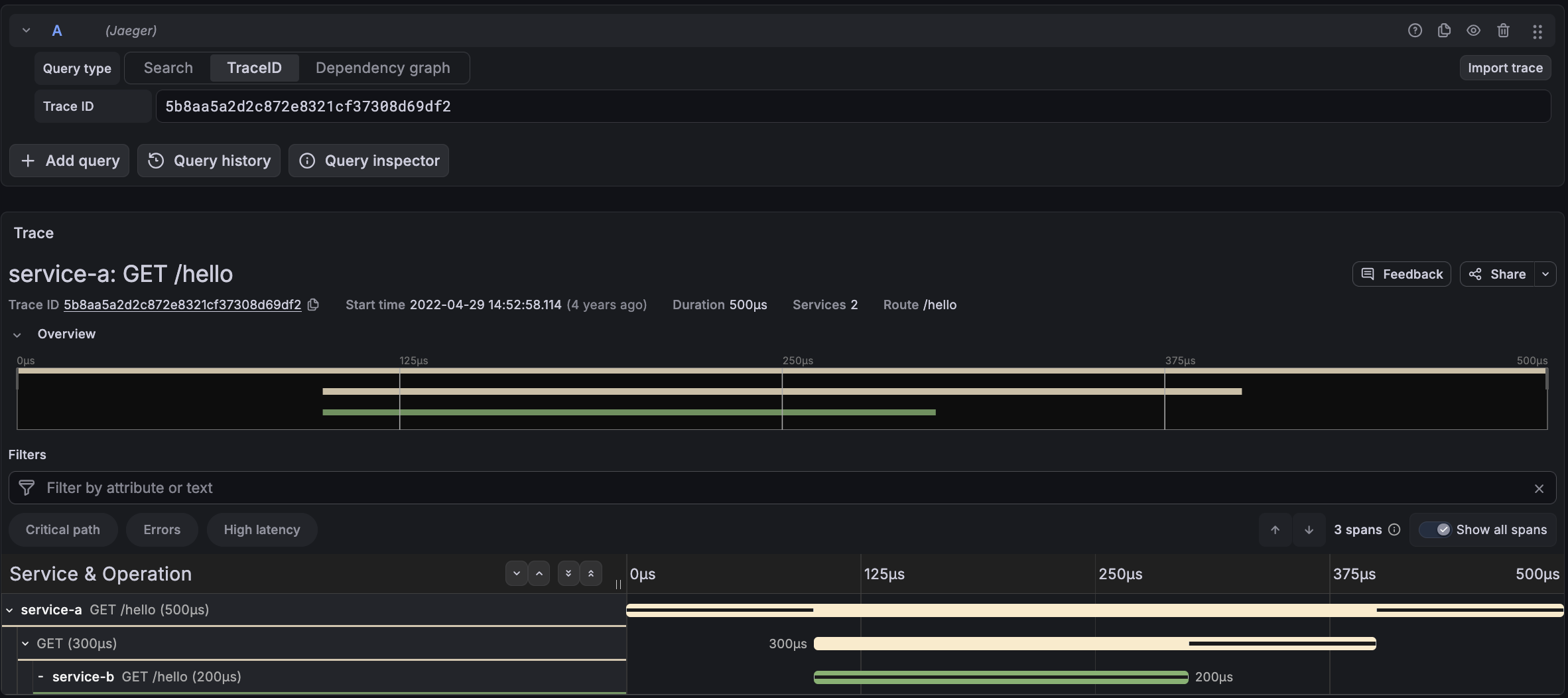
Fig. 2b — Sample Spans — The trace from $\texttt{Fig 2a}$ as represented in Jaeger

In addition to exclusive times, Siphon computes the execution pattern of each span. For a span $A$ with children $\{C_1, C_2, \ldots\}$ sorted such that $C^{\text{start}}_i \lt C^{\text{start}}_{i+1}$, adjacent children are delimited by:

• A pipe (“|”) indicates that $C_i$ happened before (in the Lamport sense) $C_{i+1}$, i.e. $A$ waited on the $C_i$ before proceeding with a call to $C_{i+1}$.

• A comma (“,”) indicates that $C_i$ and $C_{i+1}$ have overlapping execution, i.e. $A$ did not depend on the $C_i$’s result before issuing a call to $C_{i+1}$.

Calls are grouped by parentheses, and the delimiters compose recursively. The pattern "(B,C)|(D,E)" indicates that $B$ and $C$ were issued in parallel, and after both completed, $D$ and $E$ were issued in parallel. Returning to the trace in $\texttt{Fig. 2}$, the execution pattern for service A is simply "B", and the execution pattern for B is NULL (as B makes no downstream requests).

Siphon’s approach to latency estimation is quite different from existing systems. WebPerf, for example, assumes all service times are independent and carries no correlation structure through a causal graph. LatenSeer, at the other extreme, stores the joint distributions of adjacent nodes in a novel “L-Tree” data structure. Siphon supports three estimation modes, and two things set it apart: first, two of those modes fit a parametric distribution (specifically, the lognormal) to each service’s exclusive times; second, because that distribution is the lognormal, Siphon can apply a Gaussian copula trick to fold cross-service correlation into a single $n \times n$ correlation matrix.

1. Empirical Distributions, No Correlation — In this mode, services’ exclusive times are treated as independent. A method’s response time distribution is computed by convolving the empirical exclusive time distributions along a call-graph. For independent random variables, the distribution of a sum is the convolution of its summands’ distributions, which Siphon computes via FFT in $O(n \log n)$ rather than the naive $O(n^2)$.

2. Lognormal Distributions, No Correlation — In this mode, the Siphon querier asks SiphonStore for the first and second raw moments of the exclusive time distributions rather than the individual observations. This takes considerable load off the DB, network, and querier relative to mode $\textbf{(1)}$ but introduces estimation error, which compounds as we walk along the call-graph.

$\textbf{N.B}$ — The lognormal has two parameters, thus the first two raw moments exactly identify it via method of moments (see, e.g., Casella & Berger). Given empirical mean $m$ and variance $v$:

$$\begin{equation} \sigma^2 = \log\!\left(1 + \frac{v}{m^2}\right), \quad \mu = \log(m) - \frac{\sigma^2}{2} \end{equation}$$

$\textbf{TODO}$ — From experiments, we’ve observed that the KS statistic and KL divergences are quite “good” under low load. Under high load, they degrade quickly :(.

3. Lognormal Distributions, Sample Correlation Matrix — As in mode $\textbf{(2)}$, Siphon models each service’s marginal as a lognormal distribution. In this mode, Siphon encorporates cross-service dependence into its model by querying SiphonStore for an $n \times n$ correlation matrix over the $n$ services involved in a system. Rather than convolving along a call graph, Siphon samples from the copula induced by the cholesky decomposition of the correlation matrix, assigns times to each service, and walks the call graph. Because this operation is relatively inexpensive, Siphon repeates this process $m=10000$ times by default.

$\textbf{N.B}$ — If $X \sim \text{LogNormal}(\mu, \sigma^2)$, then $\ln X \sim \mathcal{N}(\mu, \sigma^2)$. Siphon further assumes that the log-transformed times are jointly Gaussian, so the joint distribution of all $n$ nodes is captured by $n$ two-parameter marginals and a single correlation matrix, rather than the $O(k^n)$ joint table a nonparametric approach would require, where $k$ is the bin-count of the quantized distribution. This is a big, loadbaring choice for Siphon and one could use a t-copula instead, as in DataDog’s TOTO, though I suspect the limitations would be similar (conjecture! 😊). As a fun fact, many attribute the 2008 Financial Crisis to a similar sort of shortcut-taking. Oops!

The reason this particular setup is worth the trouble is that the correlation structure survives the kinds of interventions Siphon needs to support. Affine transforms preserve Pearson correlation: for $a, c > 0$,

$$\begin{equation} \text{Corr}(aX + b,\, cY + d) = \frac{ac \cdot \text{Cov}(X, Y)}{ac \cdot \sqrt{\text{Var}(X)\,\text{Var}(Y)}} = \text{Corr}(X, Y) \end{equation}$$

so the correlation matrix estimated from historical traces remains valid after any affine intervention. This is what lets Siphon’s scenario model go beyond what WebPerf or LatenSeer support: LatenSeer handles translational shifts ($X' := X + b$) and pinning ($X' := b$); WebPerf handles distributional substitutions ($X' \sim F_{\theta}$), replacing a node’s distribution with one profiled under a hypothetical configuration $\theta$. Siphon subsumes the former class with arbitrary affine interventions ($X' := aX + b$) — of which translation ($a=1$) and pinning ($a=0$) are special cases — and also supports distribution substitution.

$\textbf{TODO}$ - I have to do my taxes before I get to writing up the full results. In this section, I will discuss some (encouraging) preliminary results, and then share some reasons that this method fails. In case “doing my taxes” takes 2 months (I am weak to distractions), here are some quick hints:

1. Fat tails are everywhere, for example, in TCP retransmit or Nagle’s Algorithm
2. Queue waiting time’s distort distribution shape
3. exogenous spikes distort distribution shape
4. Does a t-copula w. a YOLO’d guess for $\upsilon$ fix this? - I don’t think it’ll be that simple.
5. What situations do we get “good behavior” as the default rather than a “hard-to-achieve ideal”? State Machines? Systems that are a big pile of serverless functions? wildly over-provisioned systems?