\varphi-Accrual Failure Detection

$\varphi$ -Accrual Failure Detection

I read this paper in October of 2022 and it sent me down a rabbit hole about failure detection algorithms. In this post I will only comment on $\varphi$ -accrual, a prominent and relatively simple failure detection algorithm.

Consider two nodes $A$ and $B$ in a distributed system. Both nodes maintain a local perspective of the entire system which includes beliefs about the health of any other node. For example, $A$ may expect that the interval between messages from $B$ is distributed with some CDF, $F_B$ .

$\textbf{N.B}$ — Once again, $\textit{Casella & Berger}$ teaching me everything I know about inference. See chapter 6.2 on the sufficiency principle. Also note that we can be a bit conservative and assume the inter-arrival times follow the maximum entropy distribution (exponential) and just track the count and sum.

The code below calculates the rolling sum and rolling sum of squares of the heartbeat inter-arrival times. Along with the count of observations, these values give us enough to estimate the parameters of several common distributions (e.g. normal, uniform, exponential, etc.), if we’re okay assumung the arrival times follow a specific distribution. The original $\varphi$ -accrual paper assumes inter-arrival times are normally distributed and we will proceed as such.

$\textbf{N.B}$ — I use one of my favorite (common) numerical tricks when updating p.stats.sumSquares. If someone showed me this when I was 12 I would have started writing code much sooner. Regardless, $x^2 - y^2 = \Big(x + y)\Big(x - y)$ . In addition to being faster to compute, the RHS is also safe w.r.t catastrophic cancellation.
func Base(x, y float64) float64 {
  return math.Pow(x, 2) - math.Pow(y, 2)
}

func Safe(x, y float64) float64 {
  return (x + y) * (x - y)
}
cpu: Intel(R) Core(TM) i5-8365U CPU @ 1.60GHz
Benchmark_Mult/Base-8      36.18 ns/op
Benchmark_Mult/Safe-8      1.662 ns/op

// sample - node in a ring
type sample struct {
    value float64
    next  *sample
}

// PhiAccrualDetector - detector for each client pinging the server
type PhiAccrualDetector struct {
    stats          *SampleStatistics
    window         []sample // ring of observations
    expiringSample *sample
    lasthbts       time.Time // last heartbeat timestamp 
}

// HeartbeatHandler - update agg. statistics on each incoming heartbeat
func (p *PhiAccrualDetector) HBHandler(ctx context.Context, atime time.Time) error {
    
    var delta float64 = float64(atime.Sub(p.lasthbts) / time.Millisecond)
    var deltaExpiring float64 = p.expiringSample.value

    p.lasthbts = atime // update recent heartbeat arrival time
    p.expiringSample.value = delta // replace the oldest interval (ms) in ring
    p.expiringSample = p.expiringSample.next // prepare ptr to replace oldest val

    // update the agg. stats, collect different suff. stats (e.g. first N moments)
    // depending on estimation scheme. Normal needs count, Σ(X^2), & (ΣX)^2.
    p.stats.sum += (delta - deltaExpiring)
    p.stats.sumSquares += ((delta + deltaExpiring) * (delta - deltaExpiring))
    return nil
}

This calculation maps low probabilities to high suspicion levels. For example, with $10%, 1%, and 0.1%$ probability using $F_B$ , we have suspicion levels $1, 2, \&\ 3$ .

$\operatorname{sus}\Big(B) = -\log_{10}\Big(1 - F_{B}\Big(\textit{cur_time} - \textit{last_heartbeat}))$

N.B: $1 - F_B \in \Big(0, 1) \implies \operatorname{sus}\Big(B) \in \Big(0, \infty)$

At any moment, a client can query $A$ to get it’s $\textit{suspicion level}$ towards $B$ . The suspicion level is calculated by first calculating the probability that any heartbeat interval (assuming $F_B$ ) exceeds the current time since last heartbeat. From there, we map this value from $\Big(0, 1) \to \Big(0, \infty)$

// Suspicion - calculates suspicion given the current state and time
func (p *PhiAccrualDetector) Suspicion(ctime time.Time) float64 {
    return p.stats.Phi(p.lasthbts, ctime)
}

// SampleStats - collection of stats for calculating phi
type SampleStats struct {
    sumSquares   float64
    sum          float64
    nSamples     float64 // really an int, lazy here to avoid conversion
}

// Phi - calculate Phi (sus. level) using current offset and distribution
// implied by current interval stats
func (s *SampleStats) Phi(lastTime time.Time, curTime time.Time) float64 {

    var (
        avg float64 = (s.sum / s.nSamples)
        variance float64 = (s.sumSquares / s.nSamples) - math.Pow(avg, 2)
        tdelta float64 = float64(curTime.Sub(lastTime) / time.Millisecond)
    )

    F := 0.5 * (
        1 + math.Erf((tdelta-avg)/(math.Pow(variance, 0.5) * math.Pow(2, 0.5)))
    ) // Normal CDF
    return -math.Log10(1 - F)
}

In my experience, there are (at least) two practical problems that arise when using $\varphi$ -accrual on lossy networks:

$^{**}$ Using approximate values here, in practice $\mu_B$ is a $\textit{bit}$ larger and $\sigma_B$ a $\textit{bit}$ smaller. The point I’m making holds even with no dropped messages in the sample $F_B \sim N\Big(t, 0)$ .

On $\textit{moderately}$ lossy networks, common events can generate high suspicion levels.

Consider two $\textit{healthy}$ nodes connected by a link with constant transport time $t$ and a $1\%$ packet loss rate. Assuming a 100 sample buffer, a (very typical) sequence of messages may include a single dropped message (i.e. inter-arrival times of $t$ except for a single $2t$ ) and produce an estimate of $F_B \sim N\Big(t, t/10)^{**}$ . This scenario may lead to the detector treating a $1\%$ event as a much more rare event (via probability implied by the tails normal).
On $\textit{very}$ lossy networks, consistently poor performance can appear OK after an adjustment period.

However, if a network is sufficiently lossy (e.g. loss rate of 50%) and the buffer is small, the detector can adapt to the poor performance. After some suspicion spike, the buffer will price-in the network’s instability and report low suspicion except in the most extreme circumstances.

Naively, I suspect both of these cases can be resolved by estimating a link’s loss-rate ( $p$ ), using $F_B \sim \operatorname{Geom}\Big(p)$ or $F_B \sim \operatorname{Exp}\Big(-\ln\Big(1 - p))$ , and setting a permissible floor for $p$ .

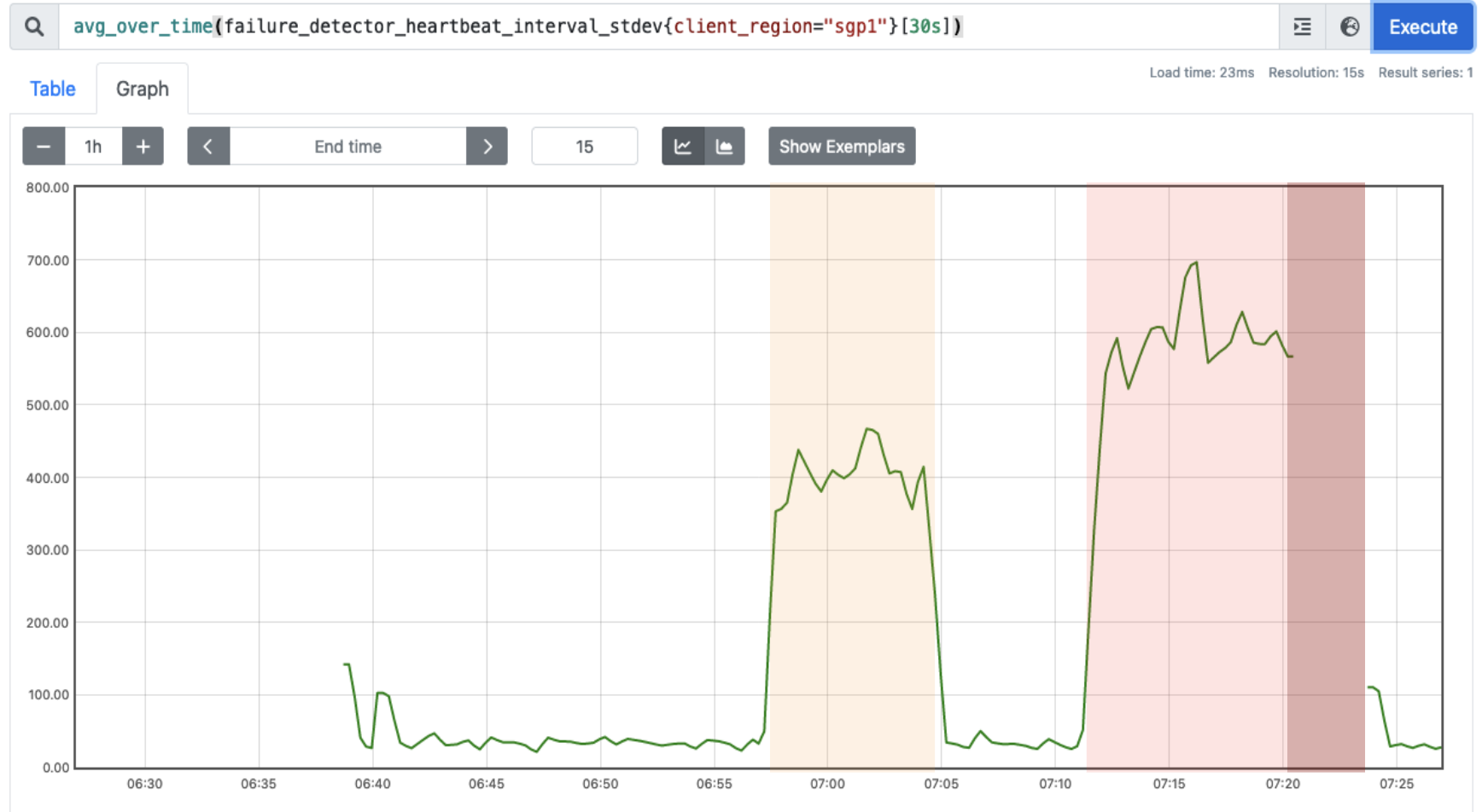
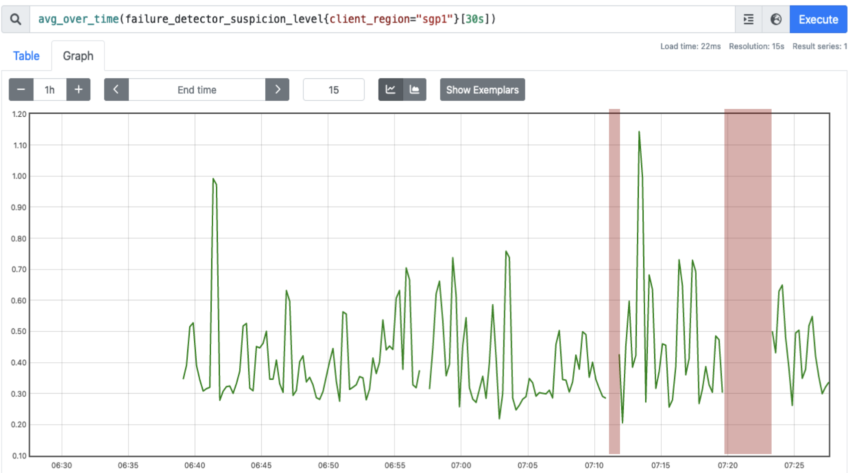
As a final note, consider the following two charts from a trial run on a somewhat unreliable (and then very unreliable) network. During the second service interruption (in light red) the suspicion level is absent (went to $+\infty$ ) for only a few seconds before the estimated CDF adjusts to the new, degraded performance level. In practice, $\varphi$ -accrual only produces consistently high suspicion levels when the node is unambiguously down.