A Few Notes On Pareto Fronts

I was in Madrid recently and skimmed On The Probability Of A Pareto Record on the plane back home. The notes below cover two questions I had about independent Pareto points. Consider $\bm{W},\bm{V} \in \mathbb{R}^d$, we say $\bm{W} \prec \bm{V}$ if $w_{i} \lt v_{i}$ for $i \in [0, d)$ and call $\bm{V}$ a pareto point of $S$ if for $\bm{W},\bm{V} \in S$, there is no point $\bm{W}$ satisfying $\bm{V} \prec \bm{W}$.

$\textbf{N.B}$ — There’s also a (very handy!) video from a Fields Institute Analysis of Algorithms conference where Fill describes the main results of On The Probability Of A Pareto Record. The bound I give in $\textbf{Q1}$ is corroborated in $\textbf{Remark 3.1}$ of the paper and briefly mentioned in the video.

$\textbf{Part 1}$ — Assuming the following, what’s the probability that the $n^{th}$ point observed is pareto?

1. Each coordinate of $\bm{V} \in \mathbb{R}^d$ is an i.i.d exponentially distributed RV.
2. Points are streamed and added to $S$ one-by-one.

Notice that $p_{n, d}$ greatly depends on the $\ell^1$ norm of $\bm{V}$. To compute the probability that a point is pareto, we integrate the product of the probability a point has $\ell^1$ norm equal to $x$ and the probability that none of the preceding $n-1$ points dominate $\bm{V}$.

$$\begin{eqnarray} p_{n,d} & = & \int_{\Omega} e^{-\|\mathbf{x}\|_1} \left(1 - e^{-\|\mathbf{x}\|_1} \right)^{n-1} \, dx \\ & = & \int_{0}^{\infty}\frac{x^{d-1}e^{-x}}{{\left(d-1\right)!}}\left(1\ -\ e^{-x}\right)^{n-1}\ dx \end{eqnarray}$$

To simplify the integral notice that the second term is strictly increasing on $\mathbb{R}^+$, and satisfies $lim_{x \to 0^+} f = 0$ and $lim_{x \to \infty} f = 1$. Thus, instead of integrating a product, we’ll just integrate the right tail of the Erlang pdf on $[n\alpha, \infty)$.

$\textbf{N.B}$ — I use $\alpha = (1 - e^{-1})^{-1} \approx 1.582$ because $F\big(n\alpha) = 0.5307$ approximates the median of the second term. I could be a bit more rigorous and integrate from $F\big(-\ln\big(1-2^{-1/(n-1)})) = 0.500$, but for $🌈\textbf{computational reasons}🌈$ we’ll be better off with the first approximation.

After zooming through a few mechanical steps we arrive at an asymptotic bound for $p_{n, d}$ that agrees with $\textbf{Remark 3.1}$ in Fill’s paper and the main result of Barndorff-Nielsen and Sobel’s On the distribution of the number of admissible points in a vector random sample.

$$\begin{equation} p_{n,d} \approx \int_{\ln\left(n\alpha\right)}^{\infty}\frac{x^{\left(d-1\right)}e^{-x}}{\left(d-1\right)!}\ dx = \frac{1}{n\alpha}\sum_{j=0}^{d-1}\frac{\ln\left(n\alpha\right)^{j}}{j!} = \Theta\left(\frac{\ln\left(n\right)^{d-1}}{ n\left(d-1\right)!}\right) \end{equation}$$

$\textbf{Part 2}$ — I’ll call the $\textbf{depth}$ of a point $\bm{V}$ in a set ($S$) the number of successive layers of pareto points that must be removed from $S$ before $\bm{V}$ becomes pareto in the remaining subset. Given $\bm{V_n}$, a newly-observed pareto point of $S$ with $\ell^1_n = \|\bm{V_n}\|_1$, what is the expected depth of $\bm{V}_n$ after an additional $m$ points are observed?

Notice that the probability of $\bm{V_n} \prec \bm{V_{j}}$ is $\prod_{i=0}^{d-1} e^{-v_n_i} = e^{-{\ell_n^1}}$. Over $m$ observations, this implies that the size of the set of points that dominate $\bm{V_n}$ is distributed by $\operatorname{Bin}(m, e^{-{\ell_n^1}})$.

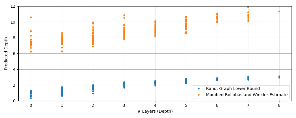
Hand-waving a bit, most pairs in this set will be non-comparable (i.e. $\bm{V_i} \nsucc \bm{V_j} \cap \bm{V_i} \nprec \bm{V_j}$) and a small fraction, $2^{-d}$, will satisfy $\bm{V_i} \prec \bm{V_j}$. If we treat the set of points that dominate $\bm{V_n}$ as a probabilistic graph, we get a lower-bound that’s logarithmic in $m$.

$$\begin{equation} \log_{2^d}\left(m \cdot e^{-\ell^1_n}\right) = \Omega\left(\frac{ln\big(m)}{d}\right) \end{equation}$$

Even better! Recall that random graphs have $\textbf{Diag}\big(G)=2 \ \textit{w.h.p}$. Voila! Done! However, our real graph has a lot more structure than one with randomly assigned edges. I’d conjecture that the actual depth of $\bm{V}_n$ is proportional to the number of layers in a non-dominating sort of the points dominating $\bm{V_n}$.

$\textbf{Update!}$ — I did what you might call “vibe-bounding” above. Fortunately for me, finding the number of layers in non-dominating sort is a research question on it’s own. When $m$ is large, this is approximately equal to the length of the longest chain from $\bm{V}_n$ to the pareto front. In The Longest Chain Among Random Points In Euclidean Space, the authors show depth is $\Theta\big(n^{1/d})$ when sampling uniformly from $[0, 1]^d$. We can map exponential coordinates to $[0, 1]^d$ easily with the CDF, but sampling uniformly from the cube may be more challenging. Let’s define $\gamma \ \colon [0, \infty)^d \to [0, 1]^d$ as the projection of $1 - e^{-\bm{X}}$ onto the diagonal of the $d$-dimensional unit cube.

$$\begin{equation} \gamma(\bm{X}) = \mathbf{1} \cdot \frac{1}{d}\sum_{i=0}^{d-1} 1 - e^{-x_i} \end{equation}$$

This transform shrinks $\ell^1_n$ (even when coordinates are transformed back into $\mathbb{R}^{+}$), but it ensures we’re considering points in the cube $[v*, 1]^d$. We now proceed with the bound proposed in Bollobás and Winkler using the point $\gamma(\bm{V_n})$ to estimate the size of the dominating set.

d = 5
b = 2 ** -d
m = 2**12
data = []

for x_n in np.random.exponential(1.0, size=(1024, d)):
    samples = np.random.exponential(size=(m, d))

    # Lower-Bound: Function of L1 norm – Assumes Random Graph
    l1_norm = np.sum(x_n)
    y0 = 1 - np.log(m) / np.log(b) + l1_norm / np.log(b)

    # Upper-Bound: Function of Transformed L1 norm
    v = transform(x_n)
    y1 = np.exp(1) * (m * np.exp(-np.sum(v))) ** (1 / d)

    # Actual: Compute Depth via Non-Dominating Sort
    dom = dominating_subset(samples, x_n) # Subset of `samples` which dominate x_n
    layers = non_dominated_sort(dom) # Claude wrote the NDS algorithm, I trust Claude, but YMMV
    x = len(layers)
    data.append((x, y0, y1))