A Sketch for One-Hit Wonder Probability From Streams

I ended my last note with two requirements for estimating a key’s one-hit wonder probability from a stream. I claimed that I needed (1) a square-integrable distribution of hits over a keyspace and (2) a space-efficient way to store an estimate of $p\big(x_k)$ for all keys. Today I’ll sketch out two alternative methods that require only the latter.

$\textbf{N.B.}$ Definitions:

Set of Possible Keys (“keyspace”): $X$

Distribution over keys $x_k \in X$ : $p\colon X \to [0, \infty)$

One Hit Wonder Prob.: $p_{ohw}\colon X \to [0, 1]$

1 — The first method reduces the scale of the problem from a calculation over $|X|$ keys to one over $n$ sets (where $n \ll |X|$ ).

2 — In my previous work I’ve used $w\big(\lambda_j, \lambda_k) = \lambda_j/\Big(\lambda_k + \lambda_j)$ to calculate the probability that a key $x_j$ arrives before $x_k$ . This method uses properties of $w$ to give a $p_{ohw}$ estimate that runs in constant time with respect to $|X|$ .

With either method, we must find the first two moments of the distribution of $w\Big(\lambda, \lambda_k)$ before producing $p_{ohw}$ . The remainder of the algorithm is quite straightforward, so today we’ll focus on how to find these moments quickly.

def pz_cache_surv_upper_bound(counts, ct_j, n_b, c=0.10):
    m_1, m_2 = calc_moments(counts, ct_j, n_b) # WANT: a _fast_ impl. of calc_moments
    theta = min(1, c / m_1)
    return ((1 - theta) * (1 - theta) * (m_1 * m_1)) / m_2

$\textbf{N.B.}$ While writing this in Go or C will improve these raw numbers, the method scales poorly as $n$ increases. This example uses $n=32$ , at $n\sim1024$ we get just $\sim3.5k\ rps$ . A few non-obvious optimizations to squeeze it down from $19\mu\text{sec} \to 12\mu\text{sec}$ /call:

Save 4 $\mu\text{sec}$ by calculating $w\big(\lambda_j, \lambda_k)$ using counts rather than probabilities. We get an equivalent result and avoid division.

Save 1.3 $\mu\text{sec}$ by replacing $\texttt{w**2}$ with $\texttt{w*w}$ .

Save 1.3 $\mu\text{sec}$ by removing check if a counter is compared with itself (i.e. avoid $\texttt{enumerate}$ ). If $n$ is large then adding $1/2n$ to the first moment is negligible. If absolutely needed, subtract from the totals on line $\texttt{8}$ .

1 — This method assumes that the hit count of a randomly-selected set of keys is a suitable proxy for the count of any key in the set.

We start by initializing $n$ counters, one for each of $n$ sets. On each $\texttt{GET}$ , we hash $x_k$ to $h\Big(x_k) \in \Big[1, n]$ and increment the corresponding counter. To be clear, we do not maintain a set of keys, we only retain the counts. When $p_{ohw}\big(x_k)$ is needed, we’ll use these counts to find a lower bound on the probability that $x_k$ ’s set is not one of the next $cn$ sets represented in the stream. In theory, if $n$ is sufficiently large (impractically large, i.e. $n \gg |X|$ ) then we can say that $h\Big(x_k)$ stores the true count $\textit{w.h.p}$ . See implementation below.

20003 function calls in 0.238 seconds # from cProfile: approx 0.09M RPS

# %lprun -f calc_moments_baseline for _ in range(20_000): calc_moments_baseline(ct_arr, 10, n_b)
Line #  Hits     Time      Per Hit   % Time  Line Contents
==============================================================
1                                           def calc_moments_baseline(ct_arr, ct_j, n_b):
2     20000    3177053.0    158.9      0.5      m_1, m_2 = 0.0, 0.0
3                                               # n.b: avoid division, don't normalize
4    660000  112742090.0    170.8     17.4      for ct_i in ct_arr: # linear w.r.t. num. bins. :(
5    640000  193703330.0    302.7     29.9          w = ct_i / (ct_j + ct_i) # division :(
6    640000  137734325.0    215.2     21.3          m_1 += w
7    640000  192782130.0    301.2     29.8          m_2 += w * w # n.b: avoid call to pow
8     20000    7414227.0    370.7      1.1      return m_1 / n_b, m_2 / n_b

Very bleak performance. I won’t pursue this method further. Luckily, we can improve on this by $\sim n$ x by making informed assumptions about the distribution of $w\big(\lambda_j, \lambda_k)$ .

2 — Let’s consider an extension of the previous approach. In the example below, I replace the loop that calculates moments with the implied moments assuming hit counts are distributed evenly across the remaining $n-1$ sets. This runs in constant time $\textit{w.r.t}$ $\Big|X|$ and can scale-up to massive keyspaces.

1000003 function calls in 0.484 seconds # from cProfile: approx 2.07M RPS (~25x !!)
# %lprun -f calc_moments_baseline_f for _ in range(20_000): calc_moments_baseline_f(10, n_b, n_req)
Line #      Hits         Time  Per Hit   % Time  Line Contents
==============================================================
1                                           def calc_moments_baseline_f(ct_j, n_b, n_req, imp_var=0.0):
2                                               # even load, x/(x+j) concave on (0,1) implies we
3                                               # overestimate m_1, var=0 impl. m_2 = m_1 * m_1
4     20000    4207325.0    210.4     30.6      u = (n_req - ct_j) / n_b 
5     20000    4444157.0    222.2     32.4      m_1 = u / (u + ct_j) # a single call to w(u, ct_j)
6     20000    5085646.0    254.3     37.0      return m_1, imp_var + (m_1 * m_1)

Uniformity in hits is a somewhat unrealistic assumption, $h$ can only balance keys across sets, not the corresponding hits.

$\textbf{Fig 1.}$ — Sets with Uniformly Dist. Keys Can Produce Unbalanced Hit Counts

Examples of bounding variance via Hoeffeding’s Lemma. If $w\big(\lambda, \lambda_j) \in \Big[\ell, \mathcal{u}]$ then variance $\leq \Big(\ell - \mathcal{u})^{2}/4$ .

Uniform Hits $\rightarrow$ constant $w\big(\lambda, \lambda_j)$ : $\operatorname{Var}=0$

Uniform $w\big(\lambda, \lambda_j)$ : $\operatorname{Var}=1/12$

Maximal Possible: $\operatorname{Var} \leq 1/4$

Very High Freq. Keys: $\operatorname{Var} \leq \big(0.5 - 1)^2/4 = 1/16$

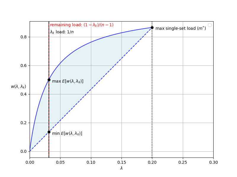
To address unequal hit counts across sets, I leave $\texttt{impl_var}$ as a parameter to be set by the application. Recall that the following relationship holds for any random variable:

$\begin{equation} \text{Var}\Big(\mathcal{X})=\int_\mathbb{R}x^{2}f\big(x)\,dx - \left(\int_{\mathbb {R} }xf\big(x)\,dx\right)^{2} \end{equation}$

If we have an opinion on the distribution of $w\Big(\lambda, \lambda_j)$ , we can set this distributions’ variance as $\texttt{impl_var}$ to arrive at the second moment without iterating over the set counts. If we so choose, we can also make the first moment configurable. The diagram below provides a visual representation of its possible values for a key with $\lambda_k = 1/n$ .

$\textbf{N.B}$ : Jensen’s gives us $\varphi\big(E\Big[X]) \geq E\big[\varphi\big(X)]$ for concave $\varphi$ . Because $w\Big(\lambda, \lambda_j)$ is concave, $w\Big(\lambda^{*}, \lambda_j)$ is the maximal first moment with $\lambda^{*} =\lambda_i = \big(1 - \lambda_j)/\big(n - 1)$ for all $i \neq j$ . If we want to really produce the lowest possible $p_{ohw}$ , then we can use $\frac{\lambda^{*}}{\lambda_j +\ m^{*}}$ given a (configurable) max single-set load of $m^{*}$ .

$\textbf{Fig 2.}$ — A Justification For Min. & Max Possible $1^{st}$ Moment

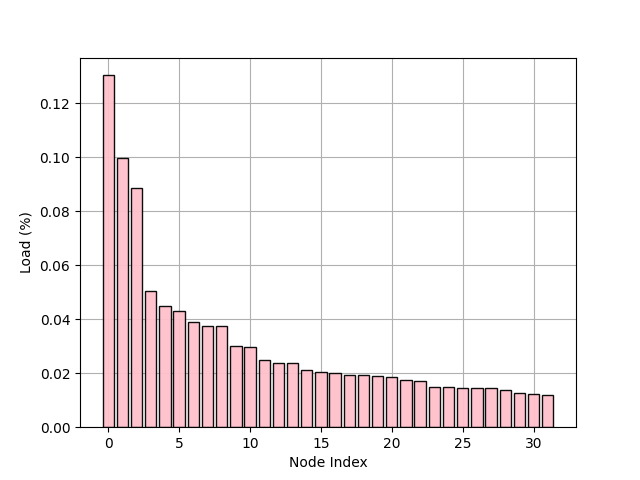
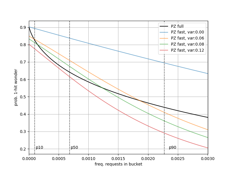
The figure below shows $p_{ohw}$ of a set with a hit-count up to the 95th percentile among $n=1024$ sets ( $1M$ total hits, $c$ =0.05). Notice that around the median hit count the values are roughly consistent with a variance around $\Big(1/16, 1/8)$ . This property isn’t universal across all distributions, but can be useful heuristic for approximating variance as a function of $\lambda_j$ .

$\textbf{Fig 3.}$ — Sets with Uniformly Distributed Keys & Unbalanced Load

To scale this method up to individual keys, I’ll simply replace the count $\texttt{ct_j}$ from the code above with a count estimated from a CountMin sketch. Unlike the array of counters proposed in 1, $\texttt{CountMinSketch}$ is a data structure that can get an approximate count $\textit{w.h.p}$ and sub-linear memory usage. I’ll wrap-up here and leave room for another note after I’ve done a more serious implementation that works in conjunction with a real LRU cache.