A Quick Note on an Inverted Index Optimization

Consider an inverted index that maps words $\omega \in \Omega$ to a postings list: the set of document IDs in which that word appears. In this scheme, IDs are assigned sequentially such that an index with $k$ documents necessarily has a document identified by each integer on $[0, k)$.

$$\begin{equation} f_{GET} \ \colon \Omega \to \mathcal{P}\big(\left[0, k\right)\big) \qquad f_{QRY} \ \colon \mathcal{P}\big({\Omega}\big) \to \mathcal{P}\big(\left[0, k\right)\big) \end{equation}$$

An operation we might be interested in performing is an intersection query. We can complete a query $Q$ with $\lvert Q \rvert$ unique words by accessing each word’s postings list and successively taking no more than $\lvert Q \rvert - 1$ set intersections. Specifically, $f_{QRY}\big(Q)$ is the intersection of all postings lists acquired by $f_{GET}\big(q)$. Perhaps this optimization is already clear to you, but I claim that in expectation, a query’s intersection cost can be improved by sorting the results of $f_{GET}$ such that postings lists are processed in increasing order.

$\textbf{N.B.}$ — I am not claiming that it’s always worth it to sort. As expected with any sort operation, we have $n\ln n$ cost. Whether this dominates the (alleged) improvement to intersection performance is up to the specific properties of the index and corpus.

Let’s start with a bound that (we will soon see) is too loose to matter. This is a false start, but perhaps it gives us some good intuition about what we need to analyze. Recall that set intersection using the standard merge algorithm has complexity $\mathcal{O}\big( \ \operatorname{min}\big( \ \lvert L \rvert, \ \lvert R \rvert \ ) \ )$, where $L$ and $R$ are the left and right operands in a foldl-style operation.

If we’ve already fetched all postings lists, we have a collection of postings lists $S$ such that $S_i := f_{GET}(q_i)$. When these postings lists are sorted by length, it follows that $\lvert L \rvert \leq \lvert R \rvert$ and therefore $\mathcal{O}\left(\sum \lvert S_i \rvert \right)$ is an upper bound. In the unsorted case, we can make a similar argument, but we can only assert that $\mathbb{E}[\lvert L \rvert] \leq \mathbb{E}[\lvert R \rvert]$. In any event, the bound $\mathcal{O}\left(\sum \lvert S_i \rvert \right)$ is still proportional to the sum of postings list sizes. Unfortunately, this result doesn’t really support the claim I’m making…

$\textbf{N.B.}$ — The last fact follows from the observation that the $j^{th}$ left operand is an intersection over $j-1$ iid draws from some distribution and the right operand is a single draw from the same distribution. Perhaps I am being too sloppy here, but I implicitly assume that the distribution of postings lists is roughly iid from an (unknown) distribution, $F$. I believe that G.K. Zipf (of the distribution) computed that English word frequency was near $Zipf(\alpha=1)$, but that’s not so helpful for us as it ignores document length and correlation.

Let’s consider an alternative argument. Because the left operand is non-increasing in size, the most conservative construction is one where $L$ remains unchanged through all $\lvert Q \rvert - 1$ folds. This occurs when the postings lists form a chain in $\big(\mathcal{P}\big([0, k)\big), \subseteq\big)$:

$$\begin{eqnarray} S_0 \subseteq S_1 \subseteq \cdots \subseteq S_{|Q|-1} \subseteq [0, k) \cap \mathbb{Z} \end{eqnarray}$$

In this case, the cost is $\mathcal{O}\big(\lvert Q \rvert \cdot \lvert S_0 \rvert\big)$. If $F$ is known, we can use order statistics to characterize $\lvert S_0 \rvert$. For example, if $F \sim \operatorname{Exp}(\lambda)$, then the minimum of $|Q|$ iid draws satisfies $S_0 \sim \operatorname{Exp}(|Q|\lambda)$, giving us a total cost bounded by $\mathcal{O}\big(|Q| \cdot \frac{1}{|Q|\lambda}\big) = \mathcal{O}\big(\lambda^{-1}\big)$. In the $\textit{unsorted}$ case, the left operand is no longer the global minimum of $|Q|$ draws but the running minimum up to the $j^{th}$ fold. This is distributed as $\sum_{j=1}^{|Q|} j\lambda e^{-j\lambda x}$. Integrating, this gives a total cost of $\mathcal{O}\big(H_{|Q|} \cdot \lambda^{-1}\big)$, where $H_{|Q|}$ is the $|Q|$-th harmonic number. In this specific case, sorting yields an improvement proportional to $\ln\big(|Q|)$. Generalizing:

$$\begin{eqnarray} \text{cost}_{\text{sorted}} &\approx& |Q| \int_0^\infty \big(1 - F(x)\big)^{|Q|}\, dx \\[4pt] \text{cost}_{\text{unsorted}} &\approx& \sum_{j=2}^{|Q|} \int_0^\infty \big(1 - F(x)\big)^{j}\, dx \end{eqnarray}$$

where $\int_0^\infty (1-F(x))^j\, dx = \mathbb{E}\big[\min(S_1, \ldots, S_j)\big]$ with all $S_i$ drawn iid from $F$.

Fortunately for us, language has structure and this chained construction’s limited improvement represents the worst-case rather than a realistic scenario. Let’s analyze the other extreme, complete independence. Consider the case where each postings list is a random sample of indexes on $[0, k)$. In this model, each document is included in a word’s postings list independently with probability $p = \mu / |\Omega|$ (where $\mu$ is the mean postings list size). In the unsorted case this yields a left operand which, in expectation, shrinks geometrically by a factor of $p$ per fold.

$$\begin{eqnarray} \mathbb{E}\big[\lvert S_0 \cap \cdots \cap S_{|Q|-1} \rvert\big] = \frac{\mu^{|Q|}}{|\Omega|^{|Q|-1}} \ \implies \ \text{cost}_{\text{unsorted}} &\approx& \sum_{j=1}^{n} \frac{\mu^j}{|\Omega|^{j-1}} \end{eqnarray}$$

Working through the algebra, we arrive at a bound of $\mathcal{O}\left( \frac{\mu}{1 - p^n} \right)$ $\approx \mathcal{O}\left(\mu\right)$. We apply a similar trick to determine the complexity of intersections of length-sorted postings lists. Let $\lvert S_0 \rvert = \textit{o}(z\mu)$ where $z \leq 1$. Applying the same analysis…

$$\begin{eqnarray} \text{cost}_{\text{sorted}} &\approx& \sum_{j=1}^{n} \frac{(z\mu)^j}{|\Omega|^{j-1}} \approx \mathcal{O}\left(z \mu \right) \end{eqnarray}$$

Finally, we do a bit of the s-word (s*mulation) to verify that the realized execution time roughly tracks the theoretical bounds. I am not a Python performance expert, I cannot defend the below as the most efficient implementation of this scheme, but I suspect it’s “close enough” to see the effects we’d like…

import functools
import numpy as np
import math
import time
import matplotlib.pyplot as plt

LAMBDA = 0.25
N_POSTINGS_LISTS = 5
N_SAMPLES = 16 * 1024
DOCUMENT_ID_SPACE_SZ = 1024

RNG = np.random.default_rng()

# This is more natural, but w.o. the early return we kinda smear performance...
# See `foldl_intersection` def'n below...
#
# def foldl_intersection(sets):
#    return functools.reduce(lambda acc, s: acc & s, sets)

def foldl_intersection(sets):
    it = iter(sets)
    try:
        acc = next(it)
    except StopIteration:
        return set()
    for s in it:
        acc &= s
        if not acc:
            return set()
    return acc
    
def chain_sampler(arr: list[int], n: int, sort: bool = False) -> list[set[int]]:
    ll = len(arr)
    bnd = RNG.exponential(ll * LAMBDA, n)
    if sort:
        bnd.sort()
    return [set(arr[:min(math.ceil(b), ll - 1)]) for b in bnd]

def unif_sampler(arr: list[int], n: int, sort: bool = False) -> list[set[int]]:
    ll = len(arr)
    bnd = RNG.exponential(ll * LAMBDA, n)
    if sort:
        bnd.sort()
    return [set(RNG.choice(ll, size=min(math.ceil(b), ll - 1), replace=False).tolist()) for b in bnd]

def time_folds(sampler, sort: bool) -> np.ndarray:
    arr = list(range(DOCUMENT_ID_SPACE_SZ))
    samples = [sampler(arr, N_POSTINGS_LISTS, sort=sort) for _ in range(N_SAMPLES)]
    times = np.empty(N_SAMPLES)
    for i, lists in enumerate(samples):
        t0 = time.perf_counter_ns()
        foldl_intersection(lists)
        times[i] = time.perf_counter_ns() - t0
    return times

fig, axes = plt.subplots(1, 2, figsize=(12, 4), sharey=True)
for ax, (name, sampler) in zip(axes, [("chain", chain_sampler), ("unif", unif_sampler)]):
    unsorted_times = time_folds(sampler, sort=False)
    sorted_times = time_folds(sampler, sort=True)
    ratio = np.median(unsorted_times) / np.median(sorted_times)

    lo = min(unsorted_times.min(), sorted_times.min())
    hi = max(unsorted_times.max(), sorted_times.max())
    bins = np.logspace(np.log10(lo), np.log10(hi), 60)

    ax.hist(unsorted_times, bins=bins, alpha=0.5, label='unsorted')
    ax.hist(sorted_times, bins=bins, alpha=0.5, label='sorted')
    ax.set_xscale('log')
    ax.set_xlabel('ns per foldl_intersection')
    if name == "chain":
        ww = math.log(N_POSTINGS_LISTS)
    else:
        ww = N_POSTINGS_LISTS
    ax.set_title(f"{name}_sampler (median ratio: {ratio:.2f}x, proj: {ww:.2f}x)")
    ax.legend()

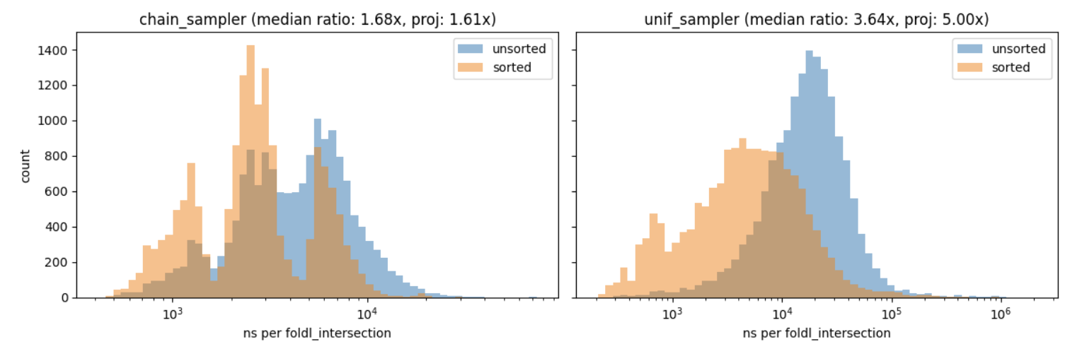
Looks “close enough” to me! We observe about a $1.68\times$ improvement vs. $\ln(5) \approx 1.61\times$ predicted. The uniform case lands at $3.64\times$ against a theoretical ceiling of $5\times$. And again, because I can’t really vouch for anything that’s going on under the hood, we ought to treat this analysis as mild supporting evidence for the bounds from earlier in the post. If I get some time later this week I’ll write a real implementation in Go or Rust.