Who Dares Make Me Balance a Binary Tree?

I started reading Alex Petrov’s Database Internals earlier this month. The first few chapters are tempting to skim through because they cover facts about data structures and databases that I suspect many readers are already familar with. With that said, there’s value in re-hashing the absolute basics. Today I’m going to solve a few problems that came to mind after reading the section on Binary Search Trees (BSTs). They share a common theme, what happens if you don’t maintain a BST?

1. Given a BST with no maintenance operation, $n$ nodes, and $l$ leaf nodes, what is the probability ($P_{\Big(n, l)}$) that we must add a level to the tree following the addition of an $n+1 ^{th}$ node?

Notice that when there are $n$ nodes in a tree there are $n+1$ slots the incoming node may occupy. Of these slots, $2l$ necessitate the addition of a new level. As a baseline estimate, $P_{\Big(n, l)} \approx 2l/\Big(n + 1)$ is probably OK. However, this implictly assumes slots are all $\frac{1}{\Big(n + 1)}$ units wide. To get an upper bound on the probability we should really study the distribution of the sizes of the slots. If we assume the BST’s values are drawn from $U\Big(0, 1)$, the slots’ sizes will have distribution $Beta\Big(1, n)$.

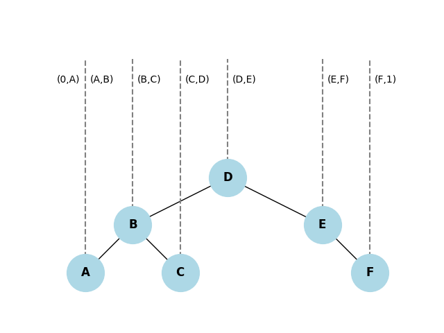
$\textbf{N.B}$ — Dubious claim about gaps of $U\Big(0, 1)^n$ that I seemingly just pulled out of thin air. See: Order Statistics Or Casella & Berger (5.4) to calm your fears. Several relevant facts:

• $U_{\Big(k)}-U_{\Big(j)}\sim Beta\Big(k-j,n-\Big(k-j)+1)$

• $Beta\Big(\alpha, \beta) = \frac{x^{\alpha-1} (1-x)^{\beta-1}}{\textbf{B}\Big(\alpha, \beta)}$

• $\textbf{B}\Big(\alpha, \beta) = \frac{\Gamma\Big(\alpha) \Gamma\Big(\beta)}{\Gamma\Big(\alpha+\beta)}$.

• $\Big(\alpha, \beta) = \Big(1, n) \implies Beta\Big(1, n) = n\Big(1-x)^{n - 1}$.

$\textbf{N.B}$ — Comparing the CDFs of $Beta\Big(1, n)$ and $Exp\Big(n)$. We can use Bernoulli’s inequality to show Beta CDF dominates Exponential CDF and $e^{-nx} > \Big(1 - x)^n \implies F_{B} \geq F_{exp}$.

• $F_{exp} = \int_0^a ne^{-nx} dx = 1 - e^{-nx}$
• $F_{B} = \int_0^a n\Big(1-x)^{n - 1} dx = 1 - (1 - x)^{n}$

The moment generating function of the Beta distribution is a disaster and I don’t want to work with it. Instead, let’s approximate $Beta\Big(1, n)$ as $Exp\Big(n)$ and take the sum of $2l$ instances of $Exp\Big(n)$ to get $P_{\Big(n, l)} \sim Gamma\Big(2l, n)$. This is a better answer, but there are (at least) two problems.

• Both $Exp\Big(n)$ and $Gamma\Big(2l, n)$ assign positive probabilty to values greater than 1.
• The sum of correlated exponential variables is $\textit{not}$ gamma distributed. The covariance between gaps of $U\Big(0, 1)^n$ can be shown to be “small” for large $n$.

Despite these transgressions, we’re just looking for a $\textit{good enough}^{TM}$ approximation. This has satisfied my curiosity, let’s move on.

2. Given a BST with no maintenance operation, can we describe the number of levels ($l$) as a function of the number of nodes ($n$)? How much worse is it than $l \sim log_2\Big(n)$?

Assume we have a $\textit{special}$ BST which has $n + 1 = 2^{\Big(l - 1)} + 1$ nodes with the first $l-1$ levels completley filled and a single node on the $l^{th}$ level. This tree does not add incoming nodes unless the new node falls in a slot which would necessitate the addition of a new level. Thus, the number of nodes needed to progress from $l$ to $l+1$ levels is exponentially distributed with parameter $2/\Big(2^{\Big(l - 1)} + 1) \approx 2^{2 - l}$. If we repeat this exercise at each level up to $l$ we end up with a series of exponential distributions:

$$\begin{equation} E\Big[R_l] \approx \sum_{k=1}^l E\Big[R_k] = \sum_{k=1}^l 2^{k - 2} = 2^{l-1} - 1/4 \end{equation}$$

When we express the equation given for $E\Big[R_l]$ (function of levels) as a function of nodes, we get $l \sim log_2\Big(n)$. Not bad! In an idealized case, our unmaintained tree performs as well as a properly maintained BST.

3. How about a more reasonable estimate? Can we get an upper bound? Can we prove a bound better than $\mathcal{O}\Big(n)$? (❌)

$\textbf{Update}$: I come with bad news. The framework I established in this section doesn’t actually provide an upper bound. Being “dense” in the upper levels actually $\textit{helps}$ us because it decreases the percentage of gaps that trigger an additional level. We can correct this by replacing $e^{-2k/n}$ with $e^{-2k/l}$ and performing the same analysis. We get Rayleigh distributions with $\sigma = \sqrt{l}$ and a bound for $l \sim n^{2/3}$. Yuck!

— DW 03.09.2024

Getting an upper bound is actually pretty easy. Unfortunatley, finding one that’s better than $\mathcal{O}\Big(n)$ is harder than I’d like. As in the previous example, we’ll assume a tree with $n + 1 = 2^{\Big(l - 1)} + 1$ nodes. This time we’ll require that each incoming node is either added to the $l^{th}$ level or necessitates the creation of level $l + 1$. The CDF for the number of nodes required for the addition of a level is as follows:

$$\begin{equation} F\Big(x) = 1 - \prod_{k=1}^{x} \Big(1 - \frac{2k}{n + k}) \end{equation}$$

Notice that $e^{-C_0k} \leq \Big(1 - \frac{2k}{n + k})$ for all $C_o \in \Big(1, \infty), k \lt n \lt \infty$. When $C_0 = 1$, we have the following approximate CDF.

$\textbf{N.B}$ — We make use of the fact that $\sum_{i=1}^j i = \frac{1}{2}\Big(j + 1)\Big(j)$.

$$\begin{equation} F\Big(x) = 1 - \prod_{k=1}^{x} e^{-k} = 1 - e^{-x\Big(x + 1)/2} \end{equation}$$

We don’t need to proceed much further to see that this CDF doesn’t depend on $n$. If our unmaintained BST behaved like this we’d have $\mathcal{O}\Big(n)$ growth. Not Good! The new goal must be to find some $C_0 \lt 1$ which can be written as a function of $n$ and produces a CDF that still dominates the BST CDF on $x \in \Big(1, n-1)$. Consider $C_0 = 2/n$.

$\textbf{Note!}$ — Chosing $C_0 = 2/n$ does not generate a CDF that dominates the BST CDF. However, $1 - e^{-2x^2/n}$ satisfies this requirement. We got lucky here…

$$\begin{equation} F\Big(x) = 1 - \prod_{k=1}^{x} e^{-2k/n} = 1 - e^{-x\Big(x + 1)/n} \leq 1 - e^{-2x^2/n} \end{equation}$$

The last inequality could probably be tightened, but this approximation gives us a nice form to work with as we finish this problem. Substituting in $n = 2^{l - 1}$, we see this is actually the Rayleigh distribution’s CDF with parameter $\sigma = 2^{\Big(l - 3)/2}$. Doing some algebra we arrive at the following sum for the expected number of nodes required to add level $l + 1$. Using $K = \sqrt{\pi / 2}$:

Rayleigh Distribution. Sleeper pick for top 10 distributions.

• Mean: $\mu = \sigma \sqrt{\pi / 2}$
• CDF: $F\Big(x) = {\displaystyle 1-e^{-x^{2}/ 2\sigma ^{2}}}$

$$\begin{equation} K \cdot \sum_{k=1}^{l} 2^{\Big(k - 3)/2} = \frac{K}{2} \Big(1 + \sqrt{2}) \Big(2^{l/2} - 1\Big) \end{equation}$$

Writing the above as a function of nodes, we arrive at our (vibes-based) upper bound of $l \sim 2 \log_2\Big(n)$.