You know Slicer and Dicer and Prancer and Vixen,
Schism and Clay and Donner and Blitzen
But do you recall
the most special dynamic sharder of them all?
I recently read a post from Databricks on their auto sharding system, Dicer. I’ve been developing a lightweight algorithm that enables dynamic sharding without the need for a dedicated coordinator service. The algorithm, which I’ve named Rudolph, shows moderately improved throughput , and reduced p99 latency when compared to traditional static hashing in exchange for a small reduction in cache efficiency ().
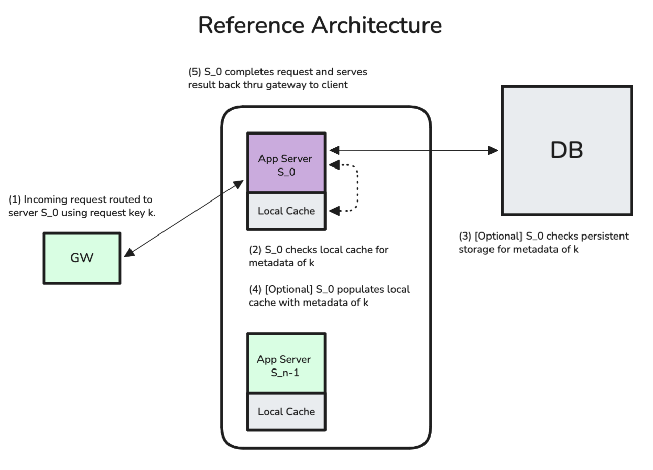
Throughout this post I’ll focus on systems with three components: a gateway server, a set of stateful application servers, and a disk-backed database with data required to process incoming requests. I assume that all application servers have the same CPU, memory, network, and other relevant constraints.
Fig. 0 - Reference Architecture — This architecture is discussed in depth in Fast key-value stores: An Idea Whose Time Has Come and Gone.
For systems with this architecture, a standard approach is to hash a relevant attribute (a request key, ) of an incoming request and route it to the server with index equal to . This method, static hashing, ensures that the same server receives similar requests as long as the number of servers is constant. Most modern proxies offer a variation on static hashing called consistent hashing, which has the helpful property of minimizing reassigned keys when the set of application servers changes. However, static hashing breaks when some request keys are much hotter than others, fixing this imbalance usually requires scaling systems out, or a separate coordination service to intelligently shard loadRudolph avoids that.
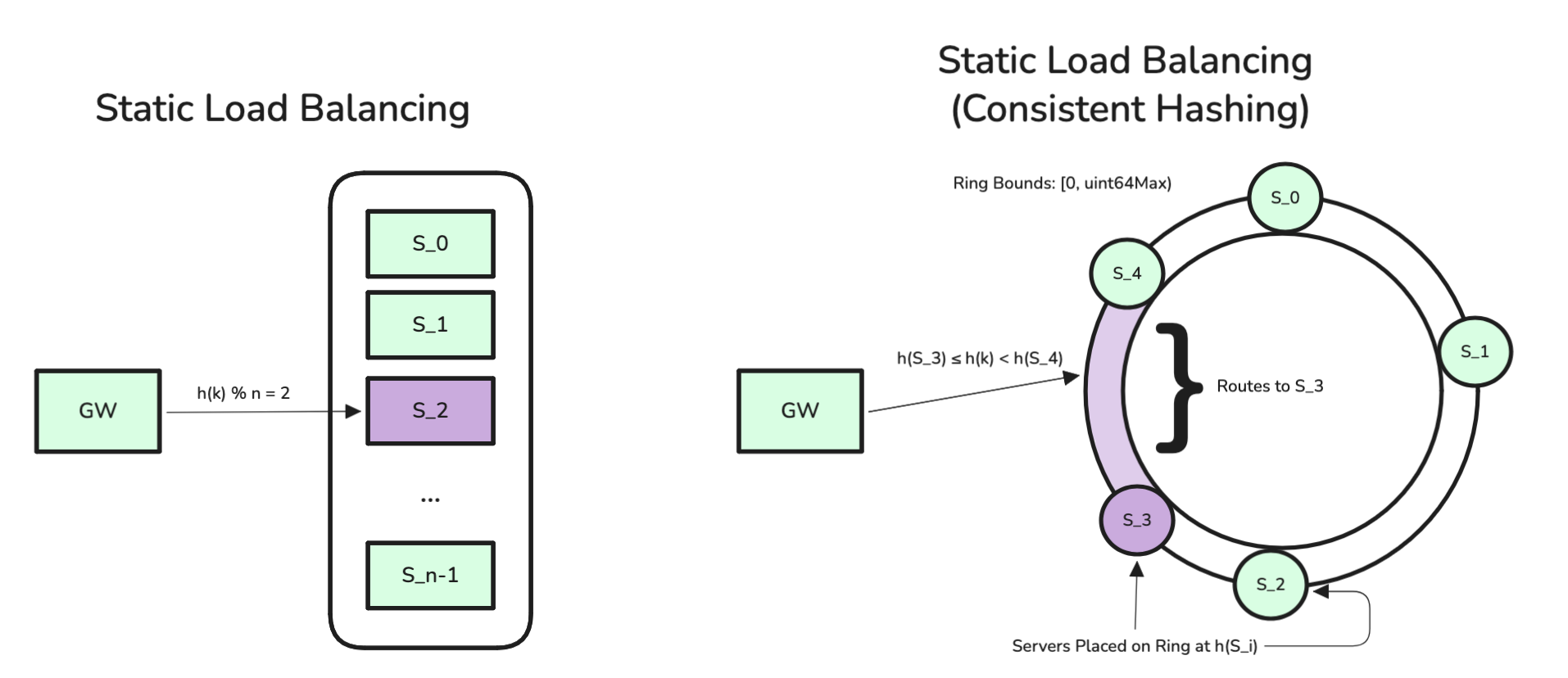
Fig. 1 - Static Hashing — Consistent hashing ensures that when a new server is added, a fraction, rather than of keys are reassigned to new servers. For additional background on consistent hashing, see D. Karger, Consistent Hashing and Random Trees.
Implicitly, static hashing assumes that requests have constant “cost” for the server to process and that the distribution of request keys is static over time. However, these assumptions break down under actual production workloads. Databricks built Dicer specifically to overcome these problems by dynamically adjusting server assignments in response to load shifts.

Fig. 2 - Dicer Architecture — See: Open Sourcing Dicer and Slicer for additional background on Dicer. See Centrifuge, Clay, and Schism for a broader background on auto sharding.
Before introducing Rudolph, I’d like to consider the purpose of systems like Dicer. Sharding systems aim to balance load across servers while preserving key affinity. Load balancing prevents any single server from becoming overloaded and key affinity maximizes the cache hit-rate which in turn minimizes DB reads. These goals are difficult to achieve simultaneously, but the job is made easier by the fact that the system does not need to achieve the optimal partitioning of request keys; a good partitioning is sufficient. There are several reasons for this.
The Search Space is Massive — The number of ways to assign unique keys to servers is the Stirling partition number, . Finding the global optimum is prohibitively expensive, so most auto sharders rely on heuristics to converge on a good partitioning.
Load is Dynamic — The optimal partitioning at time may be far from the optimal partitioning at . Because there’s no guarantee the sequence of optimal partitionings over time also preserves key affinity, it is not sufficient to only chase equalized load.
Peak Load Determines Performance — System performance is bottlenecked by the hottest server. Response latency grows nonlinearly with utilization; results from queueing theory tell us latency scales as for utilization (see Harchol-Balter, Performance Modeling and Design of Computer Systems). The goal should be minimizing peak server load, not necessarily equalizing load across all servers.
Rudolph takes these three points to the extreme and aims to minimize server load using only a small set of candidate configurations.
Rudolph is a lightweight, in-process auto sharder, a pared-down alternative to Dicer that requires no remote coordinator service. While Dicer maintains arbitrary key ranges and relies on a remote assigner to manage them, Rudolph keeps key range sizes fixed and shifts server ownership by updating a rotation parameter, . This simplification shrinks the search space from intractably large to exactly candidates, making it simple enough to run inside the gateway itself.
To initialize Rudolph for an node system, we set a small, configurable constant and a starting rotation parameter, . In the Rudolph algorithm, a request key is hashed to a bin, , and then the server is assigned as .
The gateway tracks request frequency per bin. At time , it evaluates server load under each of the possible rotations and updates to the rotation that minimizes peak server load. Regardless of , only configurations are evaluated. To avoid large jumps in , Rudolph introduces a configurable term that penalizes configurations far from the current rotation.
Example — If Rudolph were configured with bins per server, and and were approximately tied as the two best candidate rotations, we may end up oscillating between these two states, invalidating caches every few seconds. With an appropriate term, would need to yield a significant improvement to induce a shift directly from .
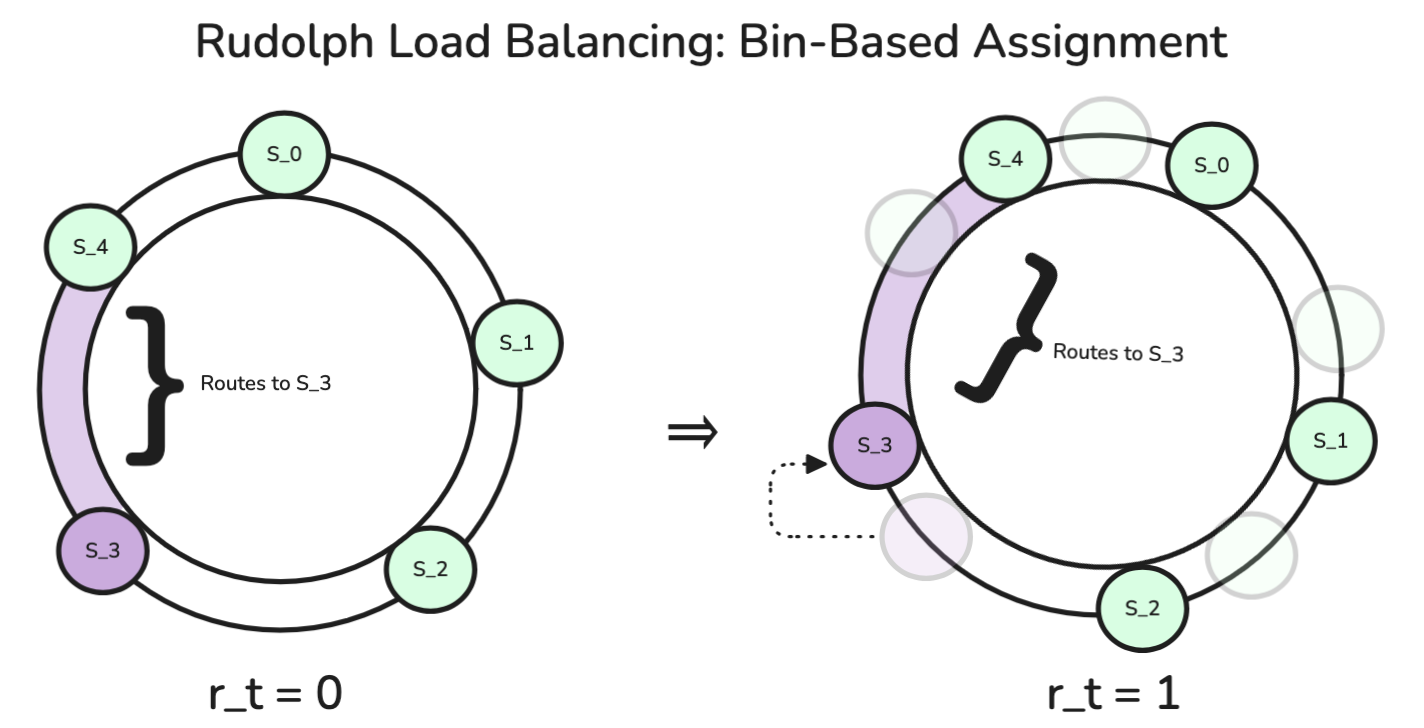
Fig. 3 - Rudolph Assignments — Rudolph partitions the keyspace into fixed bins and assigns bins to servers via rotation parameter . The purple arc shows bins owned by server under two different rotations.
| Server | ||||
|---|---|---|---|---|
| 0 | [0,4) | [1,5) | [2,6) | [3,7) |
| 1 | [4,8) | [5,9) | [6,10) | [7,11) |
| 2 | [8,12) | [9,13) | [10,14) | [11,15) |
| 3 | [12,16) | [13,17) | [14,18) | [15,19) |
| 4 | [16,0) | [17,0) ∪ [0,1) | [18,0) ∪ [0,2) | [19,0) ∪ [0,3) |
Fig. 4 - Rudolph Assignments — Assignments for , . Each column shows bin ownership under rotation . From , rotating backwards () or forwards () yield identical assignments; Rudolph would rotate backwards to minimize cache misses.
Under predictable load, Rudolph will remain on a chosen value, making only periodic, small adjustments. When initialized with sufficiently large , the algorithm effectively converges to static hashing. However, when facing traffic with shifting hotspots, Rudolph rotates away from imbalanced configurations.
To evaluate Rudolph’s performance, I ran a 15-minute test where the rotation penalty was progressively increased from to (effectively static hashing). The benchmarking workload sampled keys from a Zipfian distribution () and reshuffled every 10 seconds to create shifting hotspots. See the full implementation for details on the benchmarking setup.
As increased, throughput decreased, tail latency increased, and cache hit rate improved marginally. These results suggest that under hotspot workloads, Rudolph’s performance degrades as it converges to static hashing.
| (ms) | p50 (ms) | p90 (ms) | p99 (ms) | rps | hit (%) | |
|---|---|---|---|---|---|---|
| 0.000 | 2.60 | 2.25 | 4.83 | 8.15 | 6457 | 88.2 |
| 0.125 | 2.75 | 2.35 | 5.13 | 8.71 | 6133 | 89.2 |
| 0.500 | 2.75 | 2.36 | 5.16 | 8.64 | 6098 | 89.2 |
| 2.000 | 2.94 | 2.39 | 5.83 | 9.90 | 5885 | 90.1 |
| 8.000 | 2.97 | 2.41 | 5.93 | 9.97 | 5812 | 90.3 |
Fig. 5 - Rotation Sweep — With higher values, Rudolph converges to static hashing. Cache hit rate improves from 88.2% to 90.3% (which implies a ~12% reduction in miss rate), but throughput drops 10% and p99 latency increases 22%.
Both tail latency () and peak server load () increased with the rotation penalty. This suggests that when configured with a low rotation penalty, Rudolph successfully minimizes load on the hottest servers. Conversely, a high rotation penalty causes the algorithm to behave too rigidly. Like static hashing, it fails to avoid imbalanced configurations.
To validate Rudolph’s performance against alternative strategies, I ran a second benchmark comparing Rudolph (), static hashing, and round robin under the same workload.
| Strategy | (ms) | p50 (ms) | p90 (ms) | p99 (ms) | rps | hit (%) |
|---|---|---|---|---|---|---|
| Round Robin | 2.42 | 2.14 | 4.17 | 7.64 | 6872 | 66.5 |
| Rudolph | 2.62 | 2.26 | 4.87 | 8.28 | 6406 | 89.6 |
| Static Hash | 2.81 | 2.30 | 5.42 | 9.65 | 6157 | 90.4 |
Fig. 6.a - Strategy Comparison (Closed Benchmark) — While round robin achieves the highest total throughput, the low cache hit rate may put significant load on a DB. Rudolph improves latency metrics at the cost of only a minor decrease in cache efficiency.
| Strategy | (ms) | p50 (ms) | p90 (ms) | p99 (ms) | rps |
|---|---|---|---|---|---|
| Round Robin | 1.52 | 1.19 | 2.61 | 4.92 | 5999.83 |
| Rudolph | 1.73 | 1.41 | 3.22 | 5.26 | 5612.72 |
| Static Hash | 1.87 | 1.44 | 3.45 | 6.66 | 5391.18 |
Fig. 6.b - Strategy Comparison (Open Benchmark at 6k RPS) — Rudolph reduces p99 latency by relative to static hashing. Open benchmarks can reveal different weaknesses in a system because unlike closed-loop benchmarks, they do not have bounded concurrency. For more on benchmarking, See: B. Schroeder, Open Versus Closed: A Cautionary Tale.
These results demonstrate that Rudolph holds a position between two extremes. It sacrifices some throughput () compared to round robin to achieve much higher cache hit rates. On the other hand, it sacrifices some cache efficiency () in exchange for improved throughput and tail latency.
— What other systems sit “in the middle” between the two (sometimes conflicting) goals of maximizing throughput and maximizing cache-efficiency? Maglev and Consistent Hashing with Bounded Loads are likely the best comparisons. Like Rudolph, they both improve upon hashing-based methods without external coordination.
The round robin strategy produced the best headline numbers, but these are somewhat misleading. If DB load matters at all, round robin’s hit rate is disqualifying. Round robin would generate roughly triple the load on a hypothetical DB of the hash-based strategies. To simplify my testing procedure, my benchmarks did not even include a DB and cache misses incurred no penalty. In a system matching our reference architecture, a cache miss would likely trigger a blocking DB read and push its tail latency up.
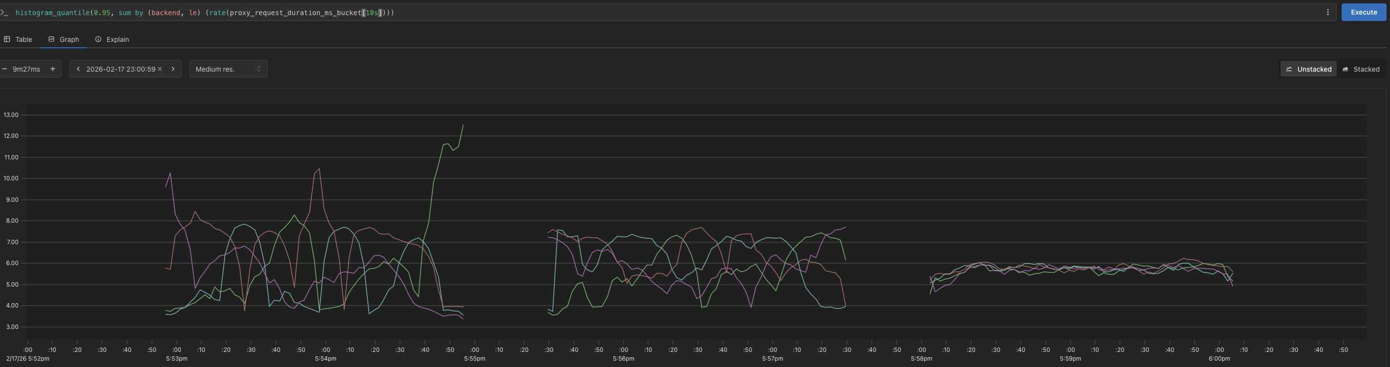
Fig. 7 - Strategy Comparison, Per-Pod p95 Latency — Static hashing (left) shows the widest pod-level variance during testing. Rudolph (middle) somewhat reduces variance, and Round robin (right) achieves the tightest distribution at the cost of additional DB load.
Overall, these tests suggest that Rudolph can augment static hashing with a degree of load-awareness. It provides an operationally simple way to add auto-sharding to a stateful system. I’ll close with a few caveats and some open questions.
Rudolph does not always improve upon static hashing. For workloads with uniform load distributions and few hotspots, static hashing is likely sufficient. While Rudolph is simpler than introducing a separate service, some effort is still required to tune and .
All experiments used a Zipfian distribution with . Analysis of production traces often shows heavier skew (i.e. , see: Clauset et al., Power-law Distributions In Empirical Data). Evaluating Rudolph under more extreme imbalance would likely yield a clearer picture of its benefits.
I haven’t addressed key migration, fault tolerance, or recovery. Systems like Dicer, with a centralized coordinator, can handle production concerns that are outside Rudolph’s scope.
The most interesting idea here may be the in-process binning approach. Nested bins (see: D. Karger) are not a novel idea, but on modern hardware, and with a reduced search space, gateways may be able to run more sophisticated placement algorithms (e.g. Least Processing Time).
I positioned Rudolph as an extension of static hashing, taking care not to compare it to consistent hashing. Implementing Rudolph as an extension of consistent hashing would be a minor lift, but could go a long way in making it more acceptable for production.
Under the LPT algorithm, we balance load by greedily assigning bins to the least loaded server. LPT keeps maximum server load down as increases, at the minor cost of maintaining a routing table with entries. LPT is known to produce a maximum load no more than , where is the best achievable balance given the bin load distribution.
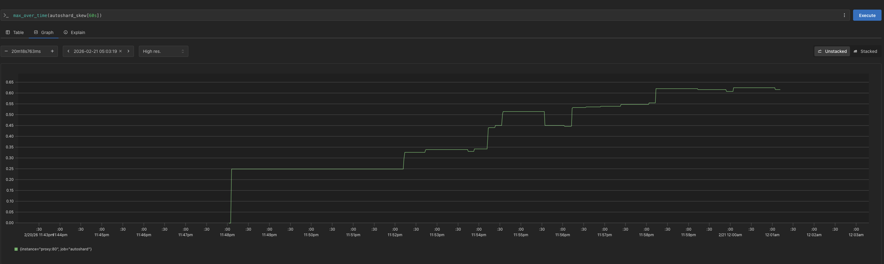
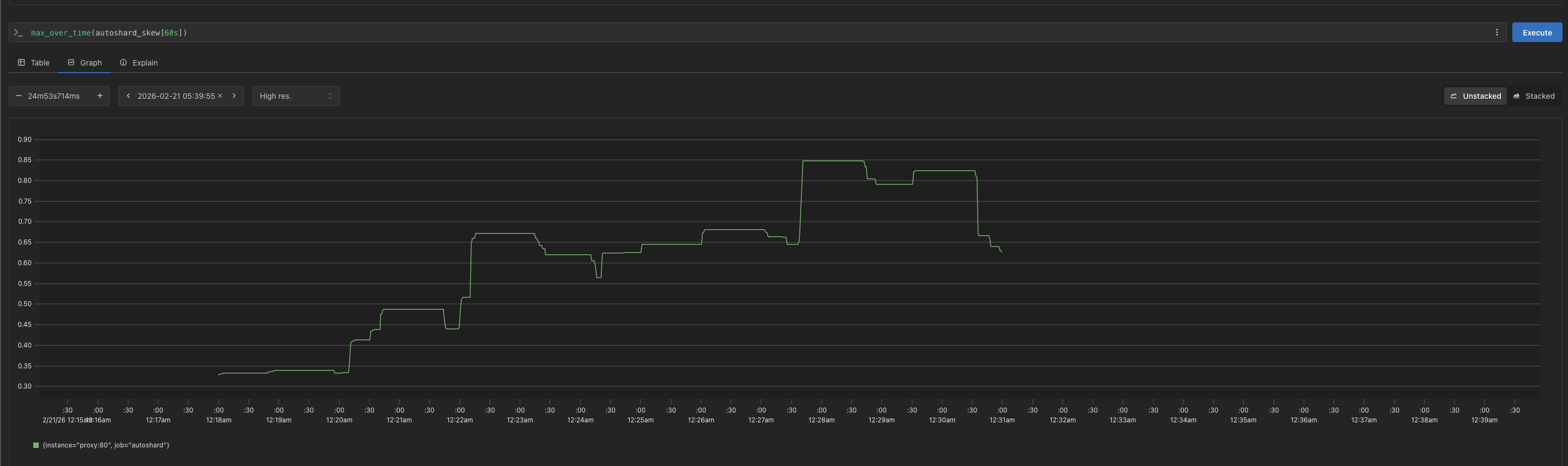
Fig. 8 - LPT Max Server Load — Both charts show max server load over a 12-minute benchmark where was ramped from to at 2-minute intervals. LPT held the maximally loaded server for the majority of the test; static hashing showed extreme imbalance from onward.
The following gives a (loose!) upper bound on expected maximum server load under random bin assignment, this is a ceiling that LPT should always improve upon. In our setting, we have a keyspace of unique request keys with weights of .
Each key is independently hashed to one of bins, this gives us an expected bin load of with for any given bin. Since the indicator variables are independent Bernoulli trials, the variance of is a weighted sum of per-key variances. We then aggregate bins per server.
Applying the Gaussian expected-maximum approximation for servers (assuming large and normality of via CLT):
As , and . At high , load concentrates on the heaviest keys, but LPT’s greedy assignment provides a reliable ceiling that static hashing doesn’t.