An Approximate Voronoi Algorithm

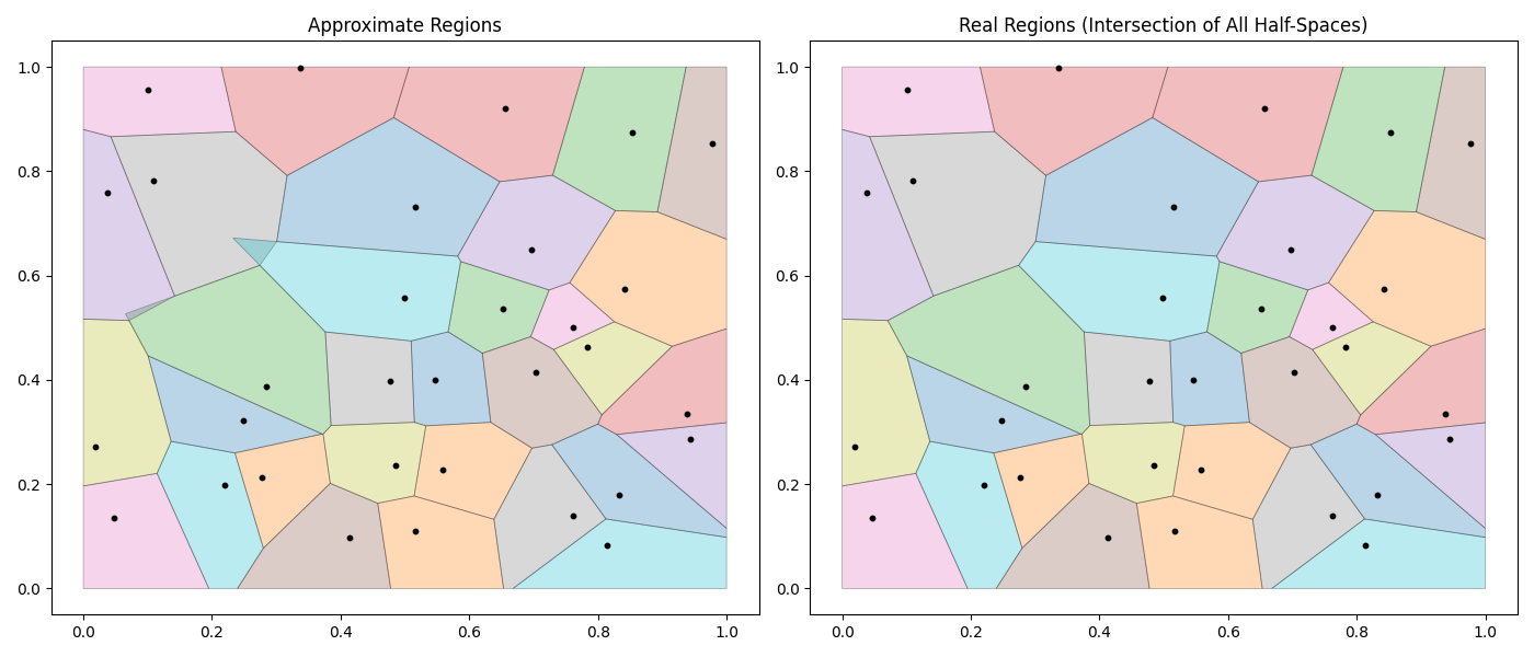
Earlier this week, I came up with an algorithm for generating approximate voronoi regions. It’s not optimal in most scenarios, but it has some nice properties:

• Lower memory footprint than Bowyer-Watson (by a constant factor around $5\times$).
• All calls to $\text{Vor}\big(s_i)$ return a superset of a site’s true voronoi region.
• $\texttt{Insert}$ and $\texttt{Delete}$ operations are $\mathcal{O}\big(c \ln n)$. This is slower than an optimized Bowyer-Watson implementation, but $c$ can be adjusted as needed and has a reasonable range around $[2, 4]$.

Consider a set of sites $S \subset \mathbb{R}^2$. We’ll store all sites in a standard quadtree; this will give us $\mathcal{O}\big(\ln n)$ inserts and deletes and $\mathcal{O}\big(\ln n + k)$ range queries. To serve queries quickly, Bowyer-Watson maintains multiple data structures to store triangulation edges and vertices. By only storing sites, our algorithm saves a good chunk of memory at the cost of needing to compute the voronoi regions on-the-fly. Determine for yourself if this is worthwhile…

For $S$ in a metric space $\big(\Omega, d)$, the voronoi region for any site $s_i$ can be computed with a series of intersections. For simplicity, we will proceed using $\mathbb{R}^2$ and Euclidean distance. With these assumptions, for each pair of sites $s_i$ and $s_j$, we can partition $\Omega$ into two half-spaces $\Omega_{ij}$ and $\Omega_{ji}$ split along the perpendicular bisector of the midpoint of $s_i s_j$. We call $\Omega_{ij}$ the side closer to $s_i$ than $s_j$.

$$\begin{equation} \text{Vor}\big(S, s_i) = \bigcap \limits_{s_k \in S, k \neq i} \Omega_{ik} \end{equation}$$

However, it is not necessary to compute $\Omega_{ij}$ for each of $n-1$ sites. The only relevant sites are the direct “neighbors” of $s_i$. It has been shown that in $\mathbb{R}^2$, regardless of $\lvert S \rvert$, the number of “neighbors” for a site is $\mathcal{O}\big(1)$ (see: notes on planar graphs). To return accurate voronoi regions, it’s sufficient to compute $\text{Vor}\big(S', s_i)$ on the set of neighbors, $S' \subseteq S$. If we select an extra non-neighbor into $S'$, doesn’t affect on the resulting region and excluding a neighbor from $S'$ will result in a region that is a superset of the true region. The problem can now be reframed as “how can we select an $S'$ that includes all ‘neighbors’ with high probability?”.

$\textbf{N.B}$ — We don’t actually know how the distribution of “neighbors” evolves as $d$ increases. Some simulation-based work has shown values for $d=3$, beyond that, information is very sparse. See simulation results - fig. 10.

I claim that if we define $S'$ as the $c\ln\big(n)$ sites nearest to $s_i$, we can produce an accurate voronoi region $\textit{w.h.p}$. Inserting a new site to the tree is $\mathcal{O}\big(\ln n)$ and computing $\text{Vor}\big(S', s_i)$ requires a $\mathcal{O}\big(\ln n + c \ln n)$ range query. Overall, this operation is $\mathcal{O}\big(c \ln n)$, and we can always recompute the region with another $\mathcal{O}\big(c \ln n)$ call to reduce overlap.

$\textbf{N.B}$ — If you read the code, you will notice that in the main text I’ve omitted the complexity of the iterative clipping step. In theory, this is $\mathcal{O}\big(c^2 \operatorname{ln}\big(n)^2)$ as each clip could add an edge. I’m hand-waving a bit here, but because we expect a constant number of “neighbors”, we also expect a constant number of vertices at each step. I believe it is safe to treat this operation as $\mathcal{O}\big(c \ln n)$. Ask yourself, do I care about the asymptotic complexity? or do we care about the constants? This isn’t a pretty algorithm, so I assume you’re here for the constants…

The cost of a delete depends on how important it is to preserve $\cup_{s_i \in S} \operatorname{Vor}\big(s_i) = \Omega$. I have mixed thoughts on this part:

• If we do not care about full coverage, this operation is just a $\mathcal{O}\big(\ln n)$ quadtree delete. If we must fill the resulting void, we’ll need to recompute $\text{Vor}\big(S', s_k)$ for some set of nearby cells.

• Assuming sites are drawn at random, I think recomputing the regions of the $c\ln\big(n)$ nearest neighbors succeeds $\textit{w.h.p}$. In this scheme, a delete is equivalent to $c\ln\big(n)$ inserts and has cost $\mathcal{O}\big(c^2\ln\big(n)^2)$.

• Recomputing the $c \ln\big(n)$ nearest neighbors may not be sufficient if the distribution of sites changes. As an alternative, I propose that when a region is first computed, we store the length of the region along its dominant axis. At delete time, we can construct a conservative estimate of the region’s bounding box and recompute the regions for all overlapping sites. This operation is equivalent to a constant number of $\mathcal{O}\big(c\ln\big(n))$ inserts.

$\textbf{N.B}$ — We must be a bit careful with the asymptotic complexities. If the density of the cell is increasing, then a delete operation can involve many sites.

I benchmarked my implementation (with a slight assist from *️⃣) on datasets of 16M and 32M sites and found we can handle up to $\sim150,000$ operations/s. This is quite slow, but perhaps it’s good enough to keep sites in memory and get just OK performance on region generation.

Benchmark_Voronoi/parallel-size=16M_neighbors=3ln(n)-8            180944              6843 ns/op
Benchmark_Voronoi/baseline-size=16M_neighbors=3ln(n)-8             52060             23019 ns/op
Benchmark_Voronoi/parallel-size=32M_neighbors=3ln(n)-8             73656             26218 ns/op
Benchmark_Voronoi/baseline-size=32M_neighbors=3ln(n)-8             24957             50666 ns/op

I ran the following program with 32M points and found it used just under 800MB. This is actually quite nice compared to the $\sim 3.2GB$ required to store sites and triangulations. Personally, if I were running some sort of large-scale logistics operation that required tracking 32M entities, I’d opt for the Bowyer algorithm and a cloud bill that’s $\$20$/month higher, but this is just my preference…

Showing nodes accounting for 796.53MB, 100% of 796.53MB total
      flat  flat%   sum%        cum   cum%
  528.02MB 66.29% 66.29%   528.02MB 66.29%  github.com/paulmach/orb/quadtree.(*Quadtree).add
  268.51MB 33.71%   100%   796.53MB   100%  main.(*VoronoiGraph).Add
         0     0%   100%   528.02MB 66.29%  github.com/paulmach/orb/quadtree.(*Quadtree).Add
         0     0%   100%   796.53MB   100%  main.main

func main() {
    go http.ListenAndServe("localhost:6060", nil)
    done := make(chan bool)

    bl, tr := orb.Point{0, 0}, orb.Point{1, 1}
    vg     := NewVoronoiGraph(orb.Bound{Min: bl, Max: tr})

    rng := rand.New(rand.NewSource(rand.Int63n(1000)))
    for i := 0; i < 32 * 1024 * 1024; i++ {
        f64x, f64y := rng.Float64(), rng.Float64()
        _ = vg.Add(f64x, f64y, 0)
    }

    for _, nn := range vg.tree.InBound(nil, orb.Bound{bl, tr}) {
        pt := nn.Point()
        id := idFromCoord(pt[0], pt[1])
        _ = vg.ApproxVoronoiCell(id, 2.0, true, nil)
    }
    <-done
}

Some final notes:

• I didn’t discuss it at all, but $\texttt{vg.ApproxVoronoiCell()}$ depends on clipping according to a variation of the Sutherland–Hodgman algorithm. This was not my focus this week, and a better implementation of this algorithm can probably cut execution time by a good deal.

• As always, I’m stubbornly refusing to use Github Gist, so the code is available here.